MATH 427: Intro to Machine Learning
Data Generating Process
Suppose we have
- Features: \(\mathbf{X}\)
- Target: \(Y\)
- Goal: Predict \(Y\) using \(\mathbf{X}\)
- Data generating process: underlying, unseen and unknowable process that generates \(Y\) given \(\mathbf{X}\)
Population
More mathematically, the “true”/population model can be represented by
\[Y=f(\mathbf{X}) + \epsilon\]
where \(\epsilon\) is a random error term (includes measurement error, other discrepancies) independent of \(\mathbf{X}\) and has mean zero.
Why Estimate \(f(\mathbf{X})\)?
We wish to know about \(f(\mathbf{X})\) for two reasons:
- Prediction: make an educated guess for what \(y\) should be given a new \(x_0\): \[\hat{y}_0=\hat{f}(x_0) \ \ \ \text{or} \ \ \ \hat{y}_0=\hat{C}(x_0)\]
- Inference: Understand the relationship between \(\mathbf{X}\) and \(Y\).
- An ML algorithm that is developed mainly for predictive purposes is often termed as a Black Box algorithm.
Prediction
There are two types of prediction problems:
- Regression (response \(Y\) is quantitative): Build a model \(\hat{Y} = \hat{f}(\mathbf{X})\)
- Classification (response \(Y\) is qualitative/categorical): Build a classifier \(\hat{Y}=\hat{C}(\mathbf{X})\)
- Note: a “hat”, \(\hat{\phantom{f}}\), over an object represents an estimate of that object
- E.g. \(\hat{Y}\) is an estimate of \(Y\) and \(\hat{f}\) is an estimate of \(f\)
Prediction and Inference
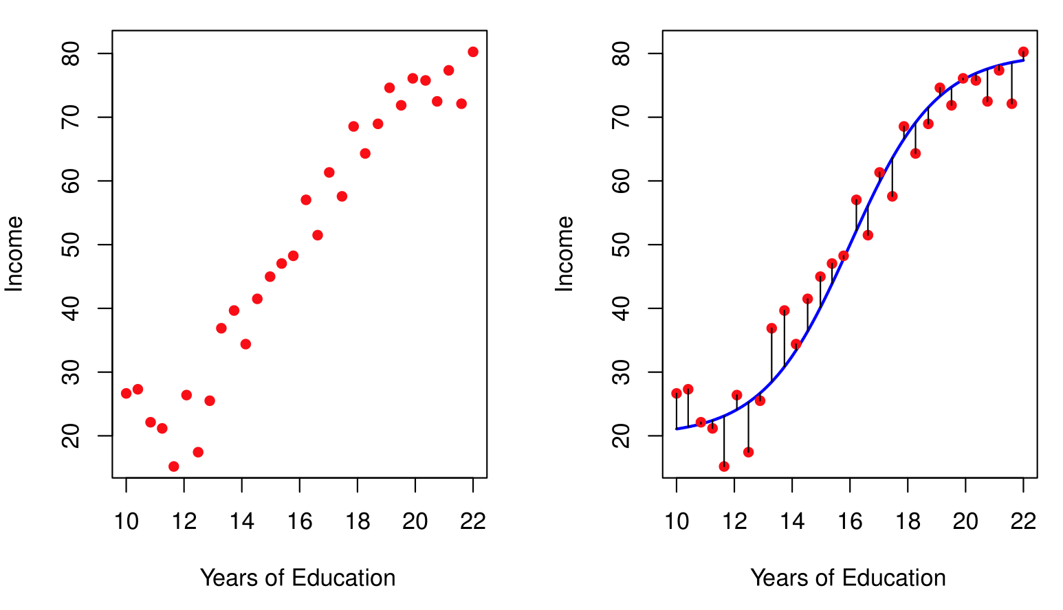
Income dataset
![]()
Why ML? (from ISLR2)
Prediction and Inference
Income dataset
Question!!!
Based on the previous two slides, which of the following statements are correct?
- As
Years of Education increases, Income increases, keeping Seniority fixed.
- As
Years of Education increases, Income decreases, keeping Seniority fixed.
- As
Years of Education increases, Income increases.
- As
Seniority increases, Income increases, keeping Years of Education fixed.
- As
Seniority increases, Income decreases, keeping Years of Education fixed.
- As
Seniority increases, Income increases.
- As
Years of Education increases, Income increases, keeping Seniority fixed. TRUE
- As
Years of Education increases, Income decreases, keeping Seniority fixed. FALSE
- As
Years of Education increases, Income increases. TRUE
- As
Seniority increases, Income increases, keeping Years of Education fixed. TRUE
- As
Seniority increases, Income decreases, keeping Years of Education fixed. FALSE
- As
Seniority increases, Income increases. TRUE
Discussion
What’s the difference between these two statements:
- As
Years of Education increases, Income increases, keeping Seniority fixed.
- As
Years of Education increases, Income increases.
How Do We Estimate \(f(\mathbf{X})\)?
Broadly speaking, we have two approaches.
- Parametric methods
- Non-parametric methods
Parametric Methods
- Assume a functional form for \(f(\mathbf{X})\)
- Linear Regression: \(f(\mathbf{X})=\beta_0 + \beta_1 \mathbf{x}_1 + \beta_2 \mathbf{x}_2 + \ldots + \beta_p \mathbf{x}_p\)
- Estimate the parameters \(\beta_0, \beta_1, \ldots, \beta_p\) using labeled data
- Choosing \(\beta\)’s that minimize some error metrics is called fitting the model
- The data we use to fit the model is called our training data
Parametric Methods
![]()
Parametric model fit (from ISLR2)
- What are some potential parametric models that could result in this picture?
- Note: Right line is the true relationship
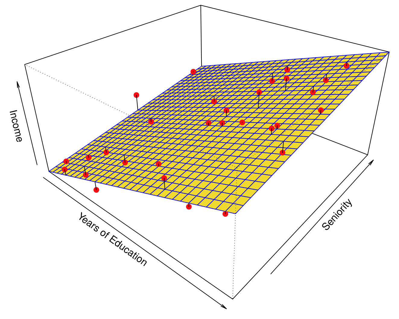
Parametric Methods
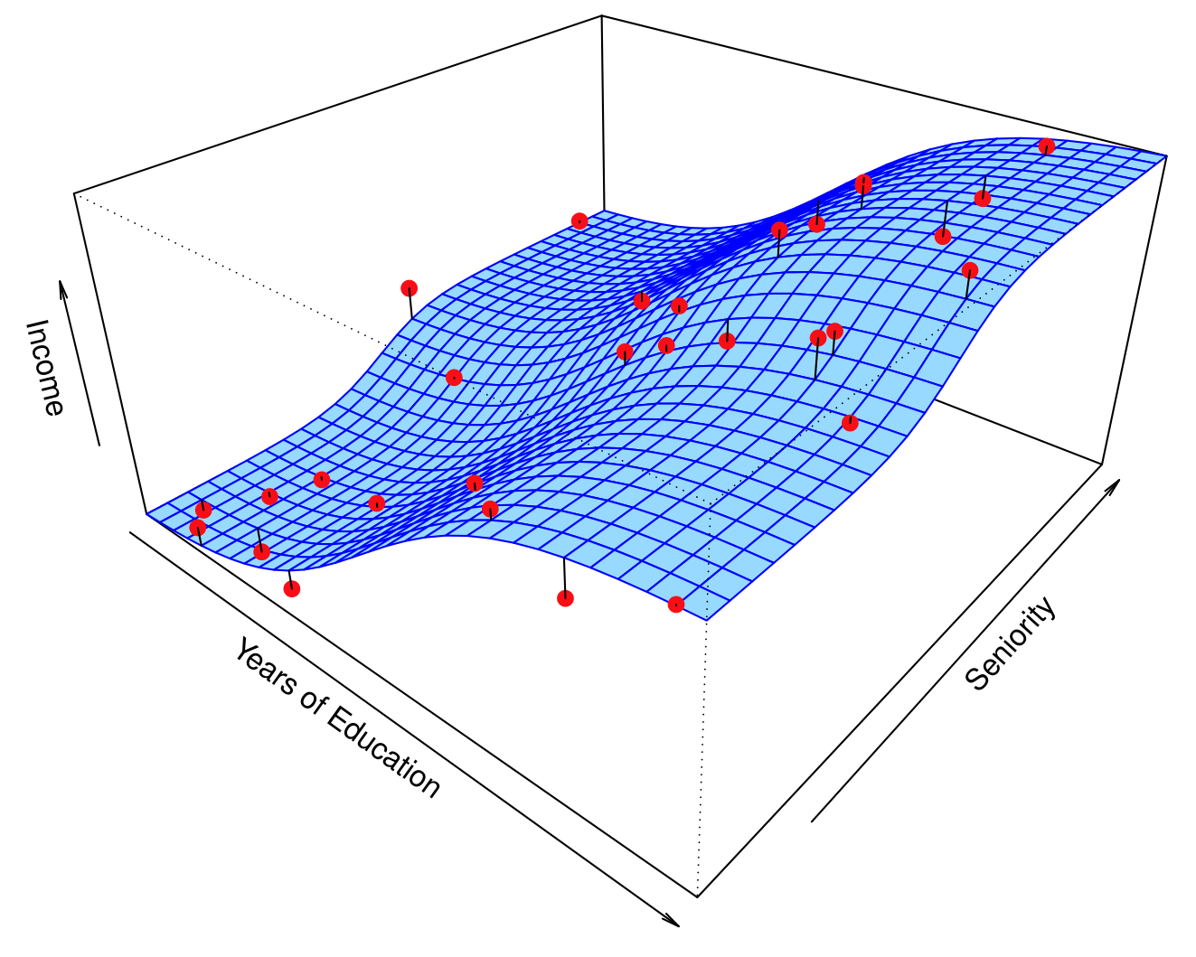
Income dataset
- What are some functions that could have resulted in the model on the right?
- \(\text{Income} \approx \beta_0 + \beta_1\times\text{Years of Education} + \beta_2\times\text{Seniority}\)
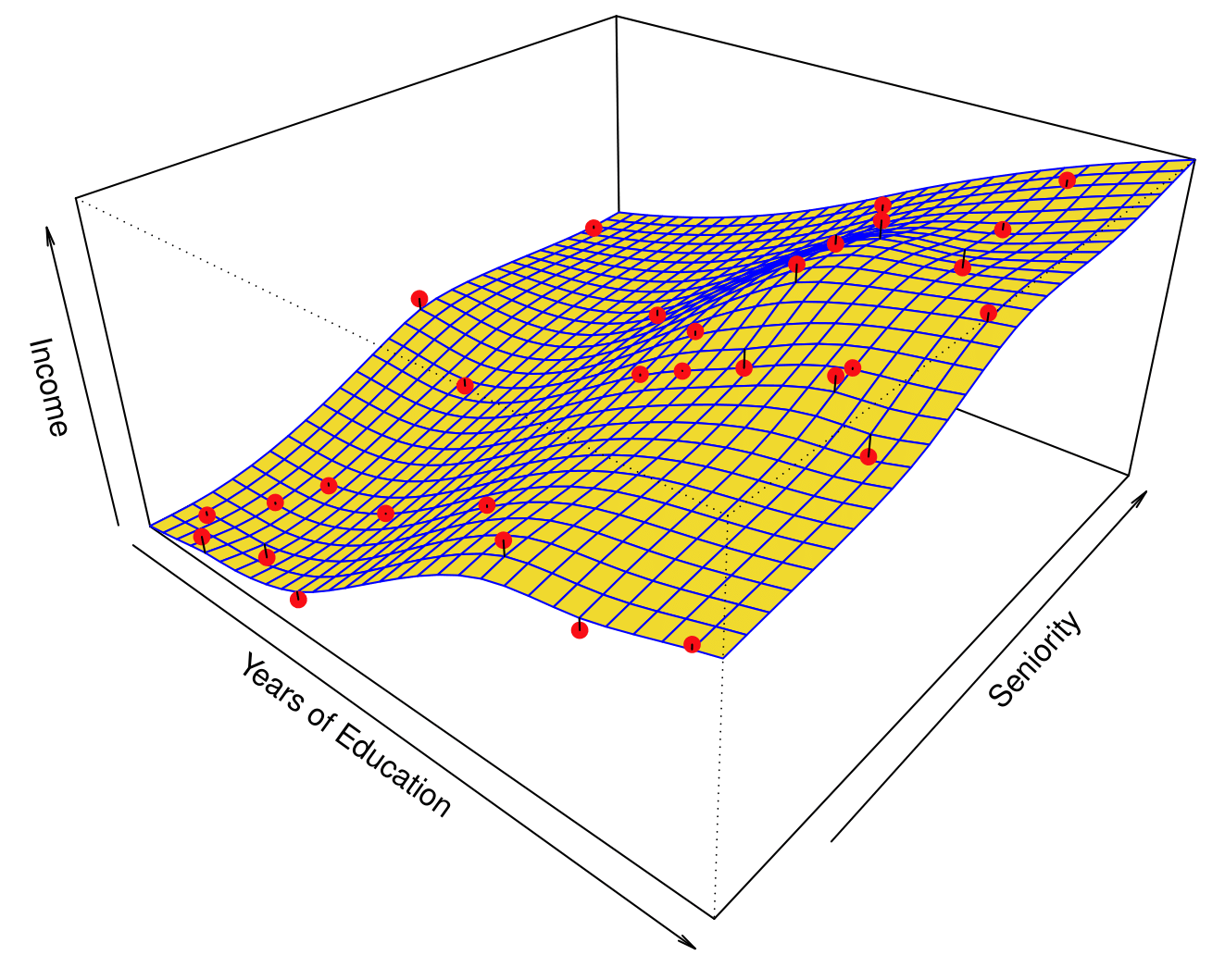
Non-parametric Methods
- Non-parametric approach: no explicit assumptions about the functional form of \(f(\mathbf{X})\)
- Much more observations (compared to a parametric approach) required to fit non-parametric model
- Idea: parametric model restricts space of possible answers
Income dataset
Supervised Learning: Flexibility of Models
- Flexibility: smoothness of functions
- More theoretically: how many parameters are there to estimate?
![]()
[More flexible \(\implies\) More complex \(\implies\) Less Smooth \(\implies\) Less Restrictive \(\implies\) Less Interpretable
Supervised Learning: Some Trade-offs
- Prediction Accuracy versus Interpretability
- Good Fit versus Over-fit or Under-fit
![]()
Trade-off between flexibility and interpretability (from ISLR2)
Supervised Learning: Selecting a Model
- Why so many different ML techniques?
- There is no free lunch in statistics: All methods have different pros and cons
- Must select correct model for each use-case
- Relevant questions in model selection:
- How much observations \(n\) and variables \(p\)?
- What is the relative importance is prediction, interpretability, and inference?
- Do we expect relationship to be non-linear?
- Regression or classification?
Recap
- Regression vs. Classification
- Parametric vs. non-parametric models
- Training v. test data
- Assessing regression models: Mean-Squared Error
- Trade-offs:
- Flexibility vs. interpretability
- Bias vs. variance