outlets <- readRDS("../data/outlets.rds")   # load dataset
head(outlets) |> kable() # first six observations of the dataset| population | profit |
|---|---|
| 6.1101 | 17.5920 |
| 5.5277 | 9.1302 |
| 8.5186 | 13.6620 |
| 7.0032 | 11.8540 |
| 5.8598 | 6.8233 |
| 8.3829 | 11.8860 |
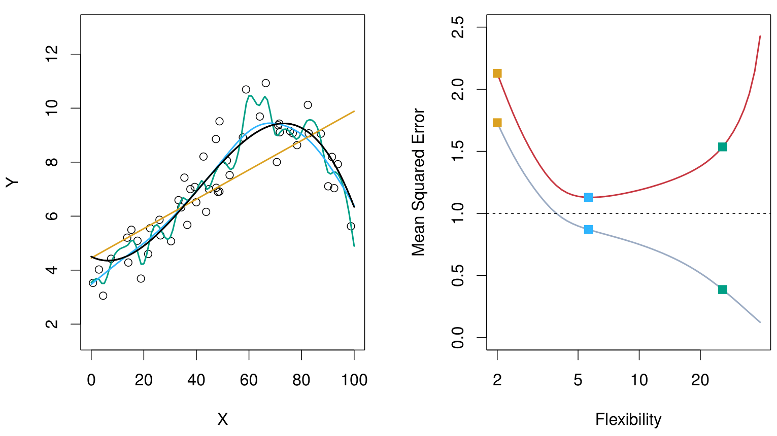
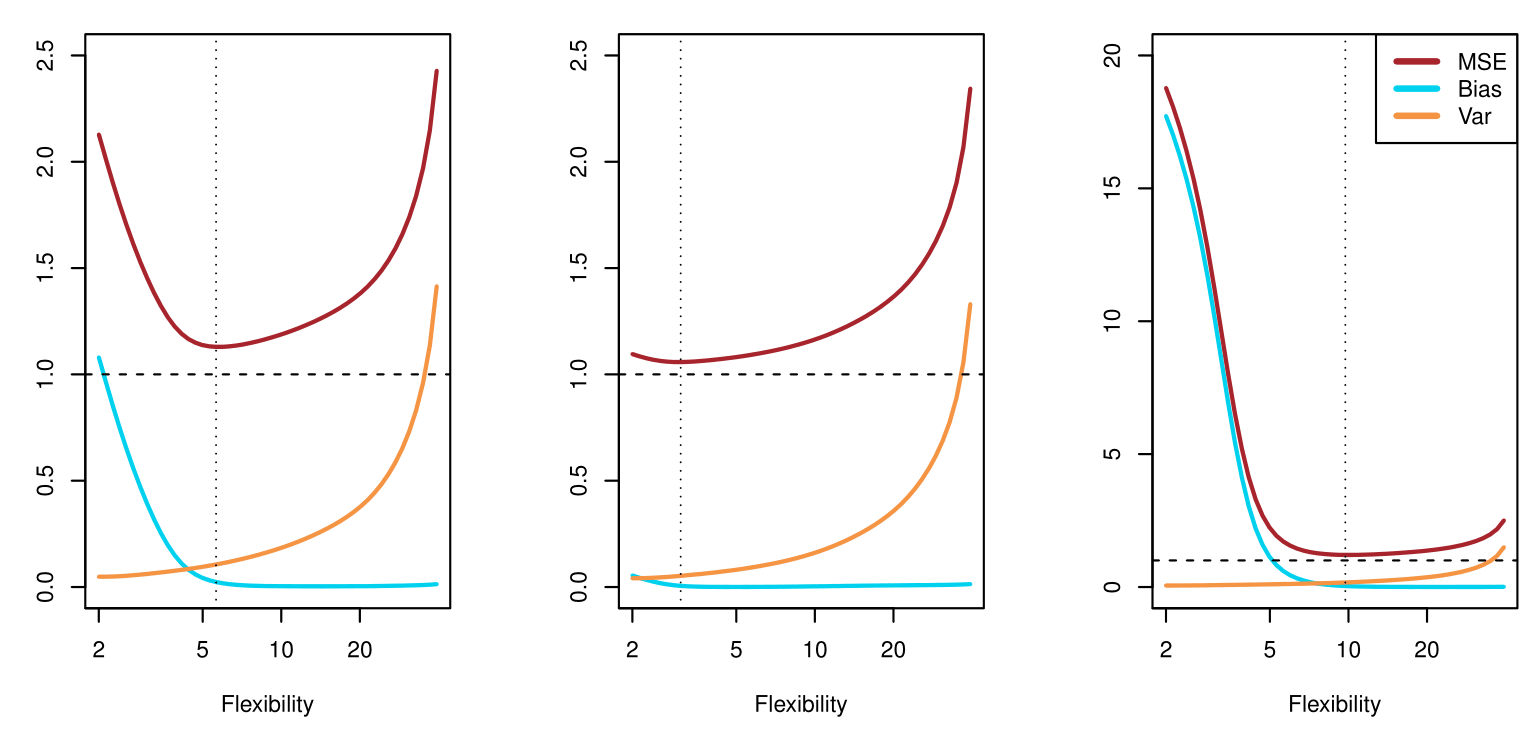
From ISLR2
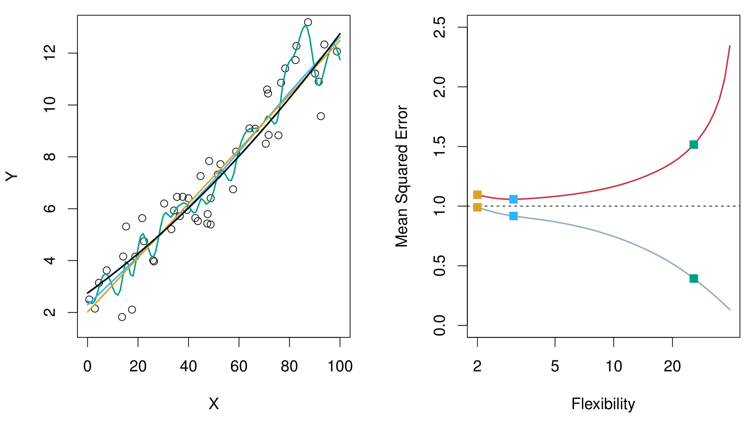
From ISLR2
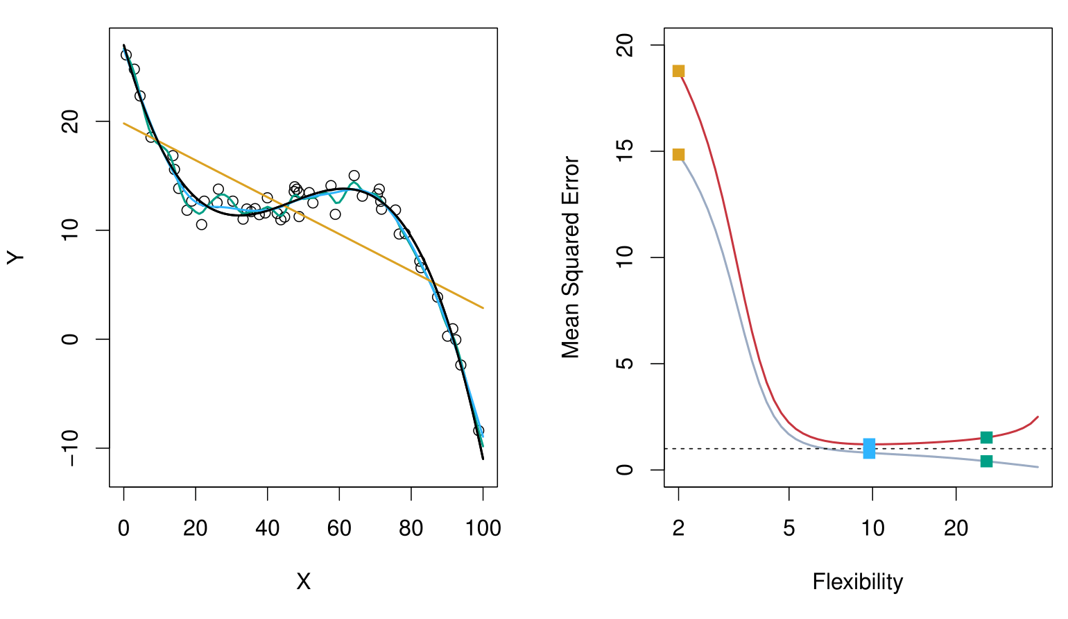
From ISLR2
From ISLR2
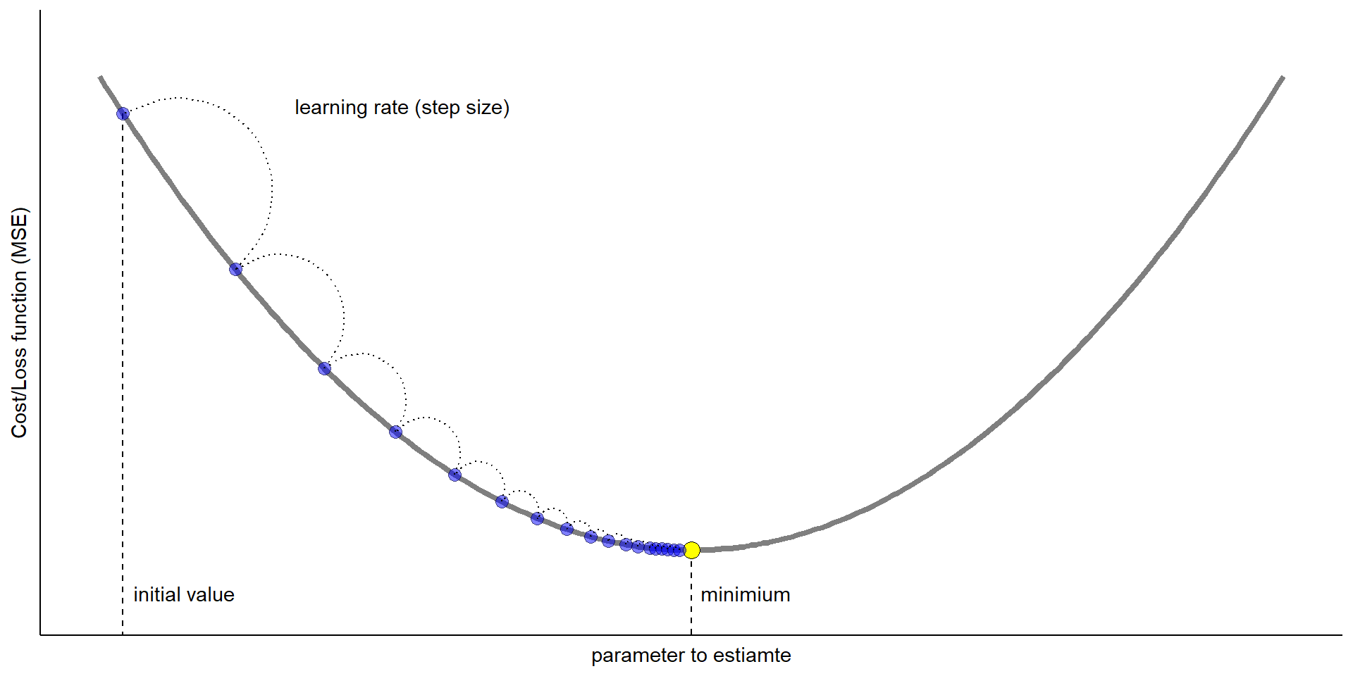
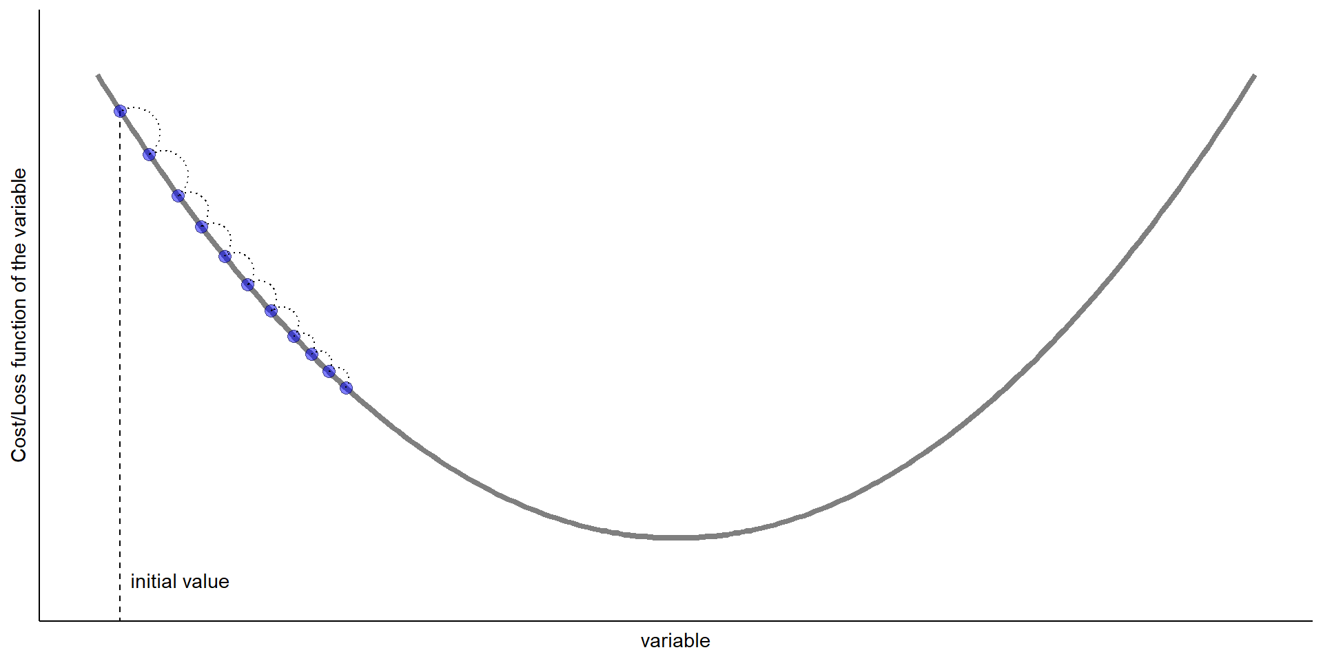
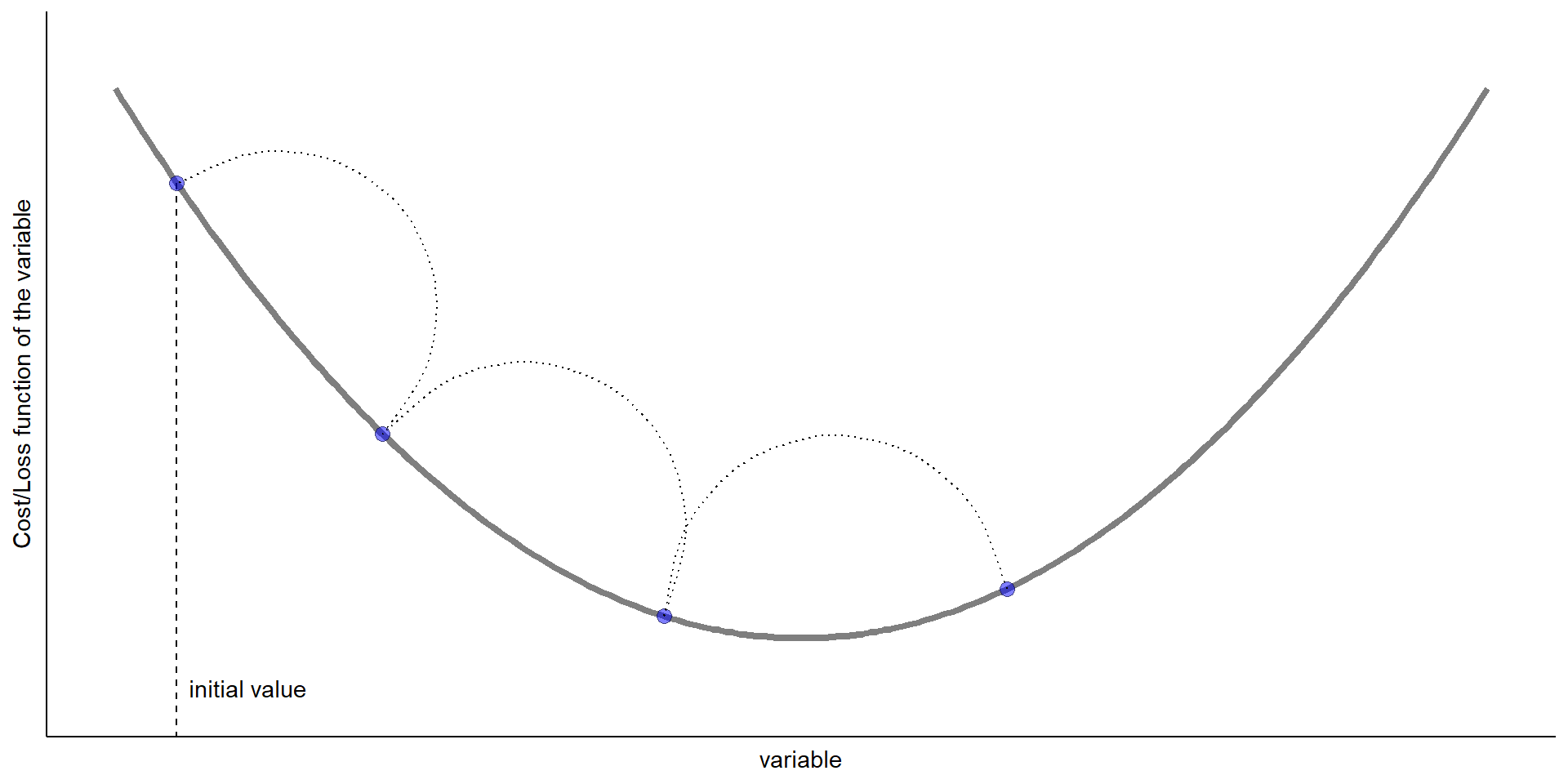
Updates to the parameter: \[ \begin{aligned} \text{new value of parameters} &= \text{old value of parameters}\\ &\qquad- \text{step size} \times \text{gradient of function w.r.t. parameters} \end{aligned} \]
![]()