MAT-427: Data Splitting + KNN

Eric Friedlander

Computational Setup

library(tidyverse)
library(tidymodels)
library(knitr)
library(readODS)
library(modeldata) # contains ames dataset

tidymodels_prefer()

mlr_model <- linear_reg() |> 
  set_engine("lm")

Comparing Models: Data Splitting

• Split ames data set into two parts
  • Training set: randomly selected proportion \(p\) (typically 50-90%) of data used for fitting model
  • Test set: randomly selected proportion \(1-p\) of data used for estimating prediction error
• If comparing A LOT of models, split into three parts to prevent information leakage
  • Training set: randomly selected proportion \(p\) (typically 50-90%) of data used for fitting model
  • Validation set: randomly selected proportion \(q\) (typically 20-30%) of data used to choosing tuning parameters
  • Test set: randomly selected proportion \(1-p-q\) of data used for estimating prediction error
• Idea: use data your model hasn’t seen to get more accurate estimate of error and prevent overfitting

Comparing Models: Data Splitting with tidymodels

set.seed(427) # Why?

ames_split <- initial_split(ames, prop = 0.70, strata = Sale_Price) # initialize 70/30
ames_split

<Training/Testing/Total>
<2049/881/2930>

ames_train <- training(ames_split) # get training data
ames_test <- testing(ames_split) # get test data

• strata not necessary but good practice
  • strata will use stratified sampling on the variable you specify (very little downside)

Linear Regression: Comparing Models

• Let’s create three models with Sale_Price as the response:
  • fit1: a linear regression model with Bedroom_AbvGr as the only predictor
  • fit2: a linear regression model with Gr_Liv_Area as the only predictor
  • fit3 (similar to model in previous slides): a multiple regression model with Gr_Liv_Area and Bedroom_AbvGr as predictors
  • fit4: super flexible model which fits a 10th degree polynomial to Gr_Liv_Area and a 2nd degree polynomial to Bedroom_AbvGr

fit1 <- mlr_model |> fit(Sale_Price ~ Bedroom_AbvGr, data = ames_train) # Use only training set
fit2 <- mlr_model |> fit(Sale_Price ~ Gr_Liv_Area, data = ames_train)
fit3 <- mlr_model |> fit(Sale_Price ~ Gr_Liv_Area + Bedroom_AbvGr, data = ames_train)
fit4 <- mlr_model |> fit(Sale_Price ~ poly(Gr_Liv_Area, degree = 10) + poly(Bedroom_AbvGr, degree = 2), data = ames_train)

Computing MSE

# Fit 1
fit1_train_mse <- mean((ames_train$Sale_Price - predict(fit1, new_data = ames_train)$.pred)^2)
fit1_test_mse <- mean((ames_test$Sale_Price - predict(fit1, new_data = ames_test)$.pred)^2)

# Fit 2
fit2_train_mse <- mean((ames_train$Sale_Price - predict(fit2, new_data = ames_train)$.pred)^2)
fit2_test_mse <- mean((ames_test$Sale_Price - predict(fit2, new_data = ames_test)$.pred)^2)

# Fit 
fit3_train_mse <- mean((ames_train$Sale_Price - predict(fit3, , new_data = ames_train)$.pred)^2)
fit3_test_mse <- mean((ames_test$Sale_Price - predict(fit3, new_data = ames_test)$.pred)^2)

# Fit 
fit4_train_mse <- mean((ames_train$Sale_Price - predict(fit4, , new_data = ames_train)$.pred)^2)
fit4_test_mse <- mean((ames_test$Sale_Price - predict(fit4, new_data = ames_test)$.pred)^2)

Question

Without looking at the numbers

1. Do we know which of the following is the smallest: fit1_train_mse, fit2_train_mse, fit3_train_mse, fit4_train_mse? Yes, fit4_train_mse
2. Do we know which of the following is the smallest: fit1_test_mse, fit2_test_mse, fit3_test_mse, fit4_test_mse? No

Choosing a Model

# Training Errors
c(fit1_train_mse, fit2_train_mse, 
  fit3_train_mse, fit4_train_mse)

[1] 6213135279 3188099910 2781293767 2472424544

which.min(c(fit1_train_mse, fit2_train_mse, 
            fit3_train_mse, fit4_train_mse))

[1] 4

# test Errors
c(fit1_test_mse, fit2_test_mse, 
  fit3_test_mse, fit4_test_mse)

[1] 6.329031e+09 3.203895e+09 2.732389e+09 2.726084e+12

which.min(c(fit1_test_mse, fit2_test_mse, 
            fit3_test_mse, fit4_test_mse))

[1] 3

• fit4 has the lowest training MSE (to be expected)
• fit3 has the lowest test MSE
  • We would choose fit3
• Anything else interesting we see?

K-Nearest Neighbors

Regression: Conditional Averaging

Restaurant Outlets Profit dataset

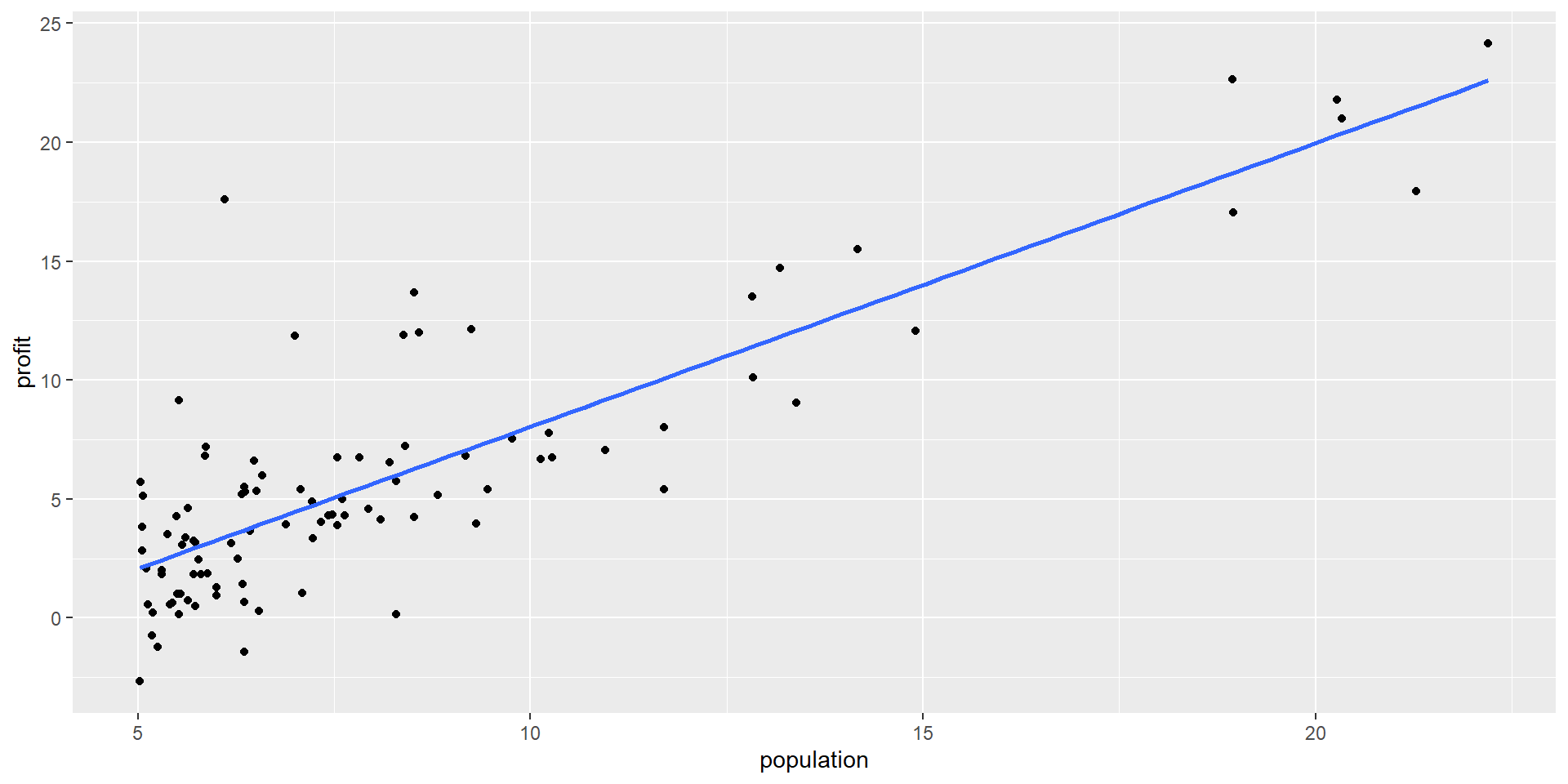
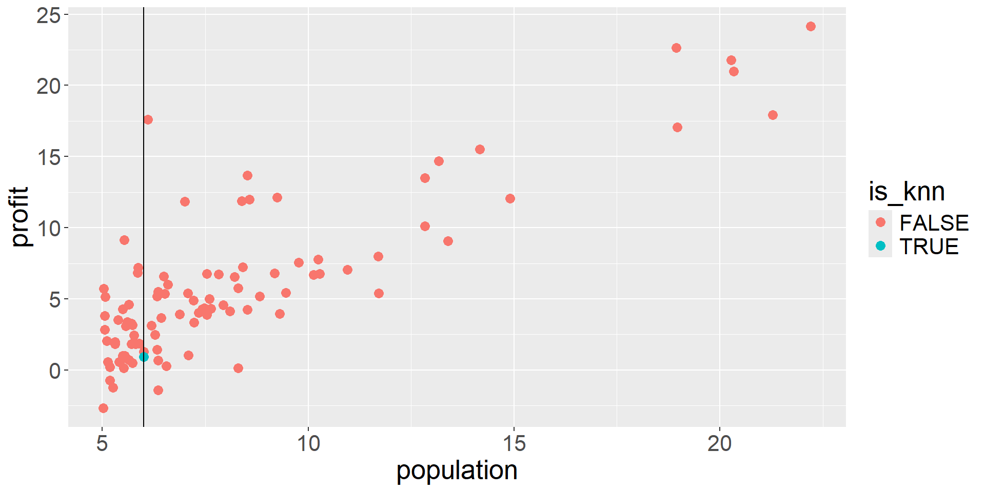
What is a good value of \(\hat{f}(x)\) (expected profit), say at \(x=6\)?

A possible choice is the average of the observed responses at \(x=6\). But we may not observe responses for certain \(x\) values.

K-Nearest Neighbors (KNN) Regression

• Non-parametric approach
• Formally: Given a value for \(K\) and a test data point \(x_0\), \[\hat{f}(x_0)=\dfrac{1}{K} \sum_{x_i \in \mathcal{N}_0} y_i=\text{Average} \ \left(y_i \ \text{for all} \ i:\ x_i \in \mathcal{N}_0\right) \] where \(\mathcal{N}_0\) is the set of the \(K\) training observations closest to \(x_0\).
• Informally, average together the \(K\) “closest” observations in your training set
• “Closeness”: usually use the Euclidean metric to measure distance
• Euclidean distance between \(\mathbf{X}_i=(x_{i1}, x_{i2}, \ldots, x_{ip})\) and \(\mathbf{x}_j=(x_{j1}, x_{j2}, \ldots, x_{jp})\): \[||\mathbf{x}_i-\mathbf{x}_j||_2 = \sqrt{(x_{i1}-x_{j1})^2 + (x_{i2}-x_{j2})^2 + \ldots + (x_{ip}-x_{jp })^2}\]

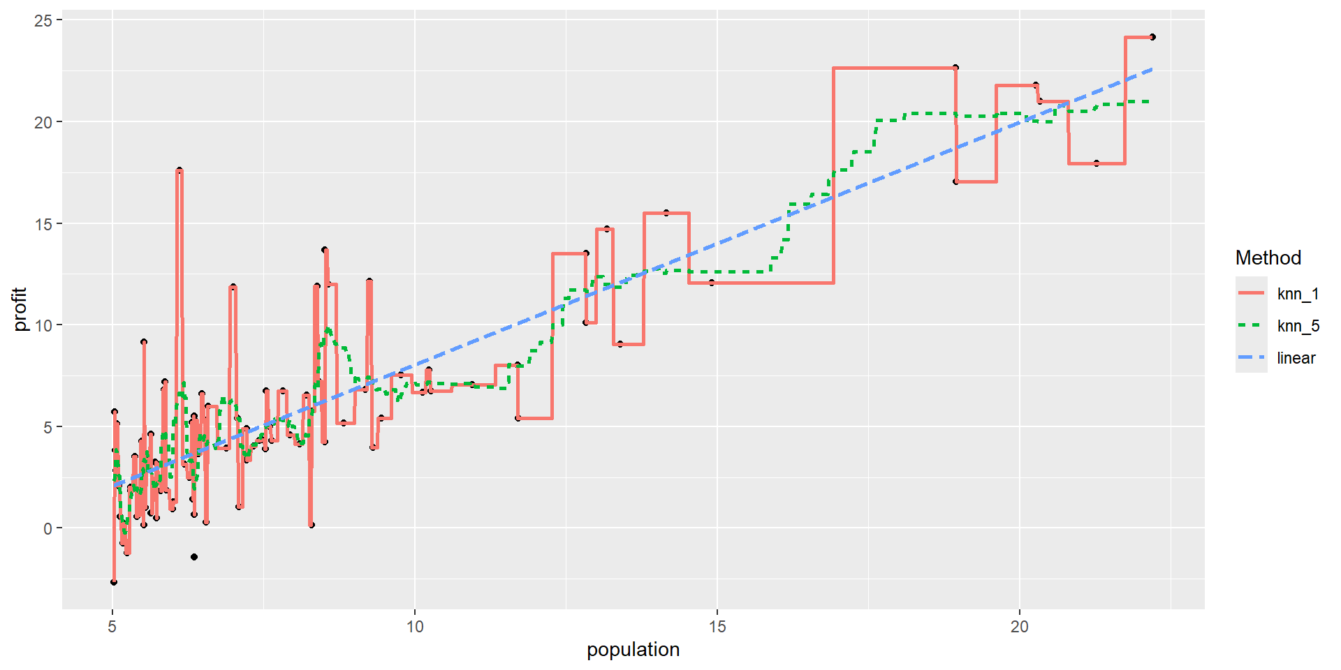
KNN Regression (single predictor): Fit

\(K=1\)

knnfit1 <- nearest_neighbor(neighbors = 1) |> 
  set_engine("kknn") |> 
  set_mode("regression") |> 
  fit(profit ~ population, data = outlets)   # 1-nn regression
predict(knnfit1, new_data = tibble(population = 6)) |> kable()  # 1-nn prediction

.pred
0.92695

\(K=5\)

knnfit5 <- nearest_neighbor(neighbors = 5) |> 
  set_engine("kknn") |> 
  set_mode("regression") |> 
  fit(profit ~ population, data = outlets)   # 1-nn regression
predict(knnfit5, new_data = tibble(population = 6)) |> kable()  # 1-nn prediction

.pred
4.113736

Regression Methods: Comparison

Question!!!

As \(K\) in KNN regression increases:

• the flexibility of the fit (decreases /increases)
• the bias of the fit (decreases/increases )
• the variance of the fit (decreases/increases)

K-Nearest Neighbors Regression (multiple predictors)

• Let’s look at the ames data

ames |>
  select(Sale_Price, Gr_Liv_Area, Bedroom_AbvGr) |>
  head() |> 
  kable()

Sale_Price	Gr_Liv_Area	Bedroom_AbvGr
215000	1656	3
105000	896	2
172000	1329	3
244000	2110	3
189900	1629	3
195500	1604	3

• Should 1 square foot count the same as 1 bedroom?
• Need to center and scale (freq. just say scale)
  • subtract mean from each predictor
  • divide by standard deviation of each predictor
  • compares apples-to-apples

Scaling in R

# scale predictors
ames_scaled <- tibble(size_scaled = scale(ames$Gr_Liv_Area),
                                  num_bedrooms_scaled = scale(ames$Bedroom_AbvGr),
                                  price = ames$Sale_Price)

head(ames_scaled) |> kable()  # first six observations

size_scaled	num_bedrooms_scaled	price
0.3092123	0.1760642	215000
-1.1942232	-1.0320576	105000
-0.3376606	0.1760642	172000
1.2073172	0.1760642	244000
0.2558008	0.1760642	189900
0.2063456	0.1760642	195500

Question…

• What about the training and test sets?
• Need to scale BOTH sets based on the mean and standard deviation of the training set…
• Discussion: Why?
• Discussion: Why don’t I need to center and scale Sale_Price?

Scaling Revisited

ames_train_scaled <- tibble(size_scaled = scale(ames_train$Gr_Liv_Area),
                                  num_bedrooms_scaled = scale(ames_train$Bedroom_AbvGr),
                                  price = ames_train$Sale_Price)

ames_test_scaled <- tibble(size_scaled = (ames_test$Gr_Liv_Area - mean(ames_train$Gr_Liv_Area)/sd(ames_train$Gr_Liv_Area)),
                                  num_bedrooms_scaled = (ames_test$Bedroom_AbvGr - mean(ames_train$Bedroom_AbvGr))/sd(ames_train$Bedroom_AbvGr),
                                  price = ames_test$Sale_Price)

• Next time: using recipe’s in tidymodels to simplify this process

K-Nearest Neighbors Regression (multiple predictors)

knnfit10 <- nearest_neighbor(neighbors = 10) |>   # 10-nn regression
  set_engine("kknn") |> 
  set_mode("regression") |> 
  fit(price ~ size_scaled + num_bedrooms_scaled, data = ames_train_scaled)

• Test Point: Gr_Liv_area = 2000 square feet, and Bedroom_AbvGr = 3, then

# obtain 10-nn prediction

predict(knnfit10, new_data = tibble(size_scaled = (2000 - mean(ames_train$Gr_Liv_Area))/sd(ames_train$Gr_Liv_Area),
                                     num_bedrooms_scaled = (3 - mean(ames_train$Bedroom_AbvGr))/sd(ames_train$Bedroom_AbvGr)))

# A tibble: 1 × 1
   .pred
   <dbl>
1 256380