| default | student | balance | income |
|---|---|---|---|
| No | No | 729.5265 | 44361.625 |
| No | Yes | 817.1804 | 12106.135 |
| No | No | 1073.5492 | 31767.139 |
| No | No | 529.2506 | 35704.494 |
| No | No | 785.6559 | 38463.496 |
| No | Yes | 919.5885 | 7491.559 |
MATH 427: Classification + Logistic Regression
Eric Friedlander
Classification Problems
- Response \(Y\) is qualitative (categorical).
- Objective: build a classifier \(\hat{Y}=\hat{C}(\mathbf{X})\)
- assigns class label to a future unlabeled (unseen) observations
- understand the relationship between the predictors and response
- Two ways to make predictions
- Class probabilities
- Class labels
Default Dataset
A simulated data set containing information on ten thousand customers. The aim here is to predict which customers will default on their credit card debt.
We will consider default as the response variable.
Split the data
Summarizing our response variable
| default | n | percent |
|---|---|---|
| No | 9667 | 0.9667 |
| Yes | 333 | 0.0333 |
| default | n | percent |
|---|---|---|
| No | 5796 | 0.966 |
| Yes | 204 | 0.034 |
| default | n | percent |
|---|---|---|
| No | 3871 | 0.96775 |
| Yes | 129 | 0.03225 |
Data Types in R
Rows: 10,000
Columns: 4
$ default <fct> No, No, No, No, No, No, No, No, No, No, No, No, No, No, No, No…
$ student <fct> No, Yes, No, No, No, Yes, No, Yes, No, No, Yes, Yes, No, No, N…
$ balance <dbl> 729.5265, 817.1804, 1073.5492, 529.2506, 785.6559, 919.5885, 8…
$ income <dbl> 44361.625, 12106.135, 31767.139, 35704.494, 38463.496, 7491.55…fct=factorwhich is the data type you want to use for categorical dataas_factorwill typically transform things (including numbers) into factors for youchrcan also be used butfactors are better because they store all possible levels for your categorical datafactors are helpful for plotting because you can reorder the levels to help you plot things
K-Nearest Neighbors Classifier
- Given a value for \(K\) and a test data point \(x_0\): \[P(Y=j | X=x_0)=\dfrac{1}{K} \sum_{x_i \in \mathcal{N}_0} I(y_i = j)\] where \(\mathcal{N}_0\) is the set of the \(K\) “closest” neighbors.
- For classification: neighbors “vote” for class (unlike in regression where predictions are obtained by averaging) \[P(Y=j | X=x_0)=\text{Proportion of neighbors in class }j\]
K-Nearest Neighbors Classifier: Build Model
- Why don’t I need to worry about centering and scaling?
K-Nearest Neighbors Classifier: Predictions
predictwith a categorical response: documentation- Two different ways of making predictions
Predicting a class
Predicting a probability
- Can anyone pick-out what’s wrong here? Hint: \(k = 10\)
I’ve been lying to you
kknnactually takes a weighted average of the nearest neighbors- I.e. closer observations get more weight
- To use unweighted KNN need
weight_func = "rectangular"
Unweighted KNN
knn_default_unw_fit <- nearest_neighbor(neighbors = 10, weight_fun = "rectangular") |>
  set_engine("kknn") |>
  set_mode("classification") |>
  fit(default ~ balance, data = default_train)   # fit 10-nn model

knn_uw_prob_preds <- predict(knn_default_unw_fit, new_data = default_test, type = "prob")   # obtain predictions as probabilities
knn_uw_prob_preds |> filter(.pred_No*.pred_Yes >0) |> head() |> kable()| .pred_No | .pred_Yes |
|---|---|
| 0.9 | 0.1 |
| 0.9 | 0.1 |
| 0.9 | 0.1 |
| 0.9 | 0.1 |
| 0.7 | 0.3 |
| 0.5 | 0.5 |
Logistic Regression
Why Not Linear Regression?
Default_lr <- default_train |>
  mutate(default_0_1 = if_else(default == "Yes", 1, 0))

lrfit <- linear_reg() |>
  set_engine("lm") |>
  fit(default_0_1 ~ balance, data = Default_lr)   # fit SLR

lrfit |> predict(new_data = default_train) |> head() |> kable()| .pred |
|---|
| 0.0316011 |
| 0.0655518 |
| -0.0065293 |
| 0.0274263 |
| 0.0451629 |
| 0.0327046 |
Why Not Linear Regression?
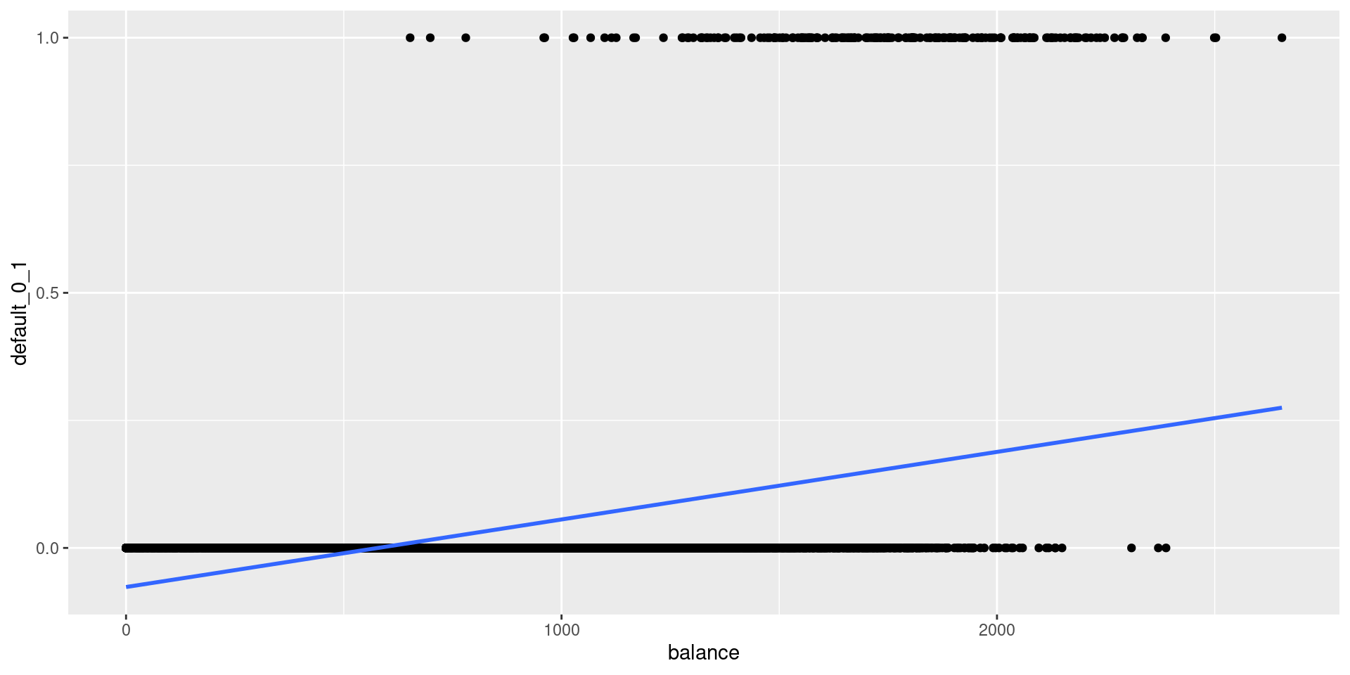
- Linear regression: does not model probabilities well
- might produce probabilities less than zero or bigger than one
- treats increase from 0.41 to 0.5 as same as 0.01 to 0.1 (bad)
Why Not Linear Regression?
Suppose we have a response, \[Y=\begin{cases} 1 & \text{if stroke} \\ 2 & \text{if drug overdose} \\ 3 & \text{if epileptic seizure} \end{cases}\]
- Linear regression suggests an ordering, and in fact implies that the differences between classes have meaning
- e.g. drug overdose \(-\) stroke \(= 1\)? 🤔
Logistic Regression
Consider a one-dimensional binary classification problem:
- Transform the linear model \(\beta_0 + \beta_1 \ X\) so that the output is a probability
- Use logistic function: \[g(t)=\dfrac{e^t}{1+e^t} \ \ \ \text{for} \ t \in \mathcal{R}\]
- Then: \[p(X)=P(Y=1|X)=g\left(\beta_0 + \beta_1 \ X\right)=\dfrac{e^{\beta_0 + \beta_1 \ X}}{1+e^{\beta_0 + \beta_1 \ X}}\]
Other important quantities
- Odds: \(\dfrac{p(x)}{1-p(x)}\)
- Log-Odds (logit): \(\log\left(\dfrac{p(x)}{1-p(x)}\right) = \beta_0 + \beta_1 \ X\)
- Linear function of predictors
Logistic Regression
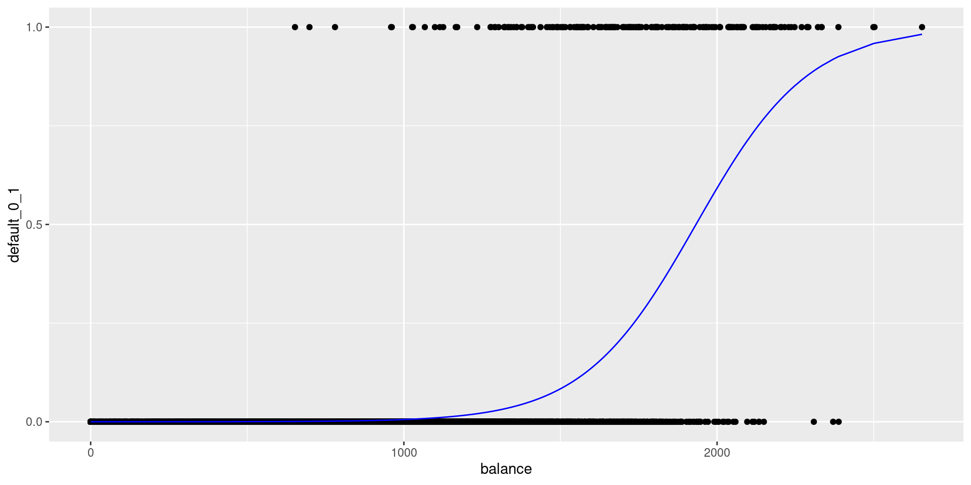
Fitting the model
Fitting a logistic regression model with default as the response and balance as the predictor:
Interpreting Coefficients
- As \(X\) increases by 1, the log-odds increase by \(\hat{\beta}_1\)
- I.e. probability of default increases but NOT linearly
- Change in the probability of default due to a one-unit change in balance depends on the current balance value
Interpreting Coefficients

Making predictions: Theory
For balance=$700,
- \[\hat{p}(X)=\dfrac{e^{\hat{\beta}_0+\hat{\beta}_1 X}}{1+e^{\hat{\beta}_0+\hat{\beta}_1 X}}=\dfrac{e^{-10.69 + (0.005533 \times 700)}}{1+e^{-10.69 + (0.005533 \times 700)}}=0.0011\]
- \[\textbf{Odds}(X) = \dfrac{\hat{p}(X)}{1-\hat{p}(X)} = \dfrac{0.0011}{1-0.0011}\approx 0.0011\]
- \[\textbf{Log-Odds}(X)=\log\left(\dfrac{\hat{p}(X)}{1-\hat{p}(X)}\right) = \log(0.0011) = -6.80\]
Making predictions in R
predict(logregfit, new_data = tibble(balance = 700), type = "class") |> kable() # obtain class predictions| .pred_class |
|---|
| No |
predict(logregfit, new_data = tibble(balance = 700), type = "raw") |> kable() # obtain log-odds predictions| x |
|---|
| -6.819727 |
predict(logregfit, new_data = tibble(balance = 700), type = "prob") |> kable() # obtain probability predictions| .pred_No | .pred_Yes |
|---|---|
| 0.9989092 | 0.0010908 |