MATH 427: Evaluating Classification Models

Eric Friedlander

Tips on Gradient Descent HW

  • Make step size small!
  • May take a while to converge
  • Try adaptive step size (i.e. backtracking)
  • Clarification on stopping criteria
    • Set tolerance
    • Stop when distance from gradient to \((0, 0)\) is below tolerance

Computational Set-Up

library(tidyverse)
library(tidymodels)
library(gridExtra)
library(janitor) # for next contingency tables
library(kableExtra)
library(ISLR2)

tidymodels_prefer()

Default Dataset

A simulated data set containing information on ten thousand customers. The aim here is to predict which customers will default on their credit card debt.

head(Default) |> kable()  # print first six observations
default student balance income
No No 729.5265 44361.625
No Yes 817.1804 12106.135
No No 1073.5492 31767.139
No No 529.2506 35704.494
No No 785.6559 38463.496
No Yes 919.5885 7491.559

Response Variable: default

Default |> 
  tabyl(default) |>  # class frequencies
  kable()           # Make it look nice
default n percent
No 9667 0.9667
Yes 333 0.0333

Split the data

set.seed(427)

default_split <- initial_split(Default, prop = 0.6, strata = default)
default_split
<Training/Testing/Total>
<6000/4000/10000>
default_train <- training(default_split)
default_test <- testing(default_split)

K-Nearest Neighbors Classifier: Build Model

  • Response (\(Y\)): default
  • Predictor (\(X\)): balance
knnfit <- nearest_neighbor(neighbors = 10) |> 
  set_engine("kknn") |> 
  set_mode("classification") |>  
  fit(default ~ balance, data = Default)   # fit 10-nn model

K-Nearest Neighbors Classifier: Predictions

predict(knnfit, new_data = Default, type = "class") |> head() |> kable()   # obtain predictions as classes
.pred_class
No
No
No
No
No
No
  • Predicts class w/ maximum probability
predict(knnfit, new_data = Default, type = "prob") |> head() |> kable() # obtain predictions as probabilities
.pred_No .pred_Yes
1 0
1 0
1 0
1 0
1 0
1 0

Fitting a logistic regression

Fitting a logistic regression model with default as the response and balance as the predictor:

logregfit <- logistic_reg() |> 
  set_engine("glm") |> 
  fit(default ~ balance, data = default_train)   # fit logistic regression model

tidy(logregfit) |> kable()  # obtain results
term estimate std.error statistic p.value
(Intercept) -10.6926385 0.4659035 -22.95033 0
balance 0.0055327 0.0002841 19.47329 0

Making predictions in R

predict(logregfit, new_data = tibble(balance = 700), type = "class") |> kable()   # obtain class predictions
.pred_class
No
predict(logregfit, new_data = tibble(balance = 700), type = "raw") |> kable()   # obtain log-odds predictions
x
-6.819727
predict(logregfit, new_data = tibble(balance = 700), type = "prob") |> kable()  # obtain probability predictions
.pred_No .pred_Yes
0.9989092 0.0010908

Assessing Performance of Classifiers

Binary Classifiers

  • Start with binary classification scenarios
  • With binary classification, designate one category as “Success/Positive” and the other as “Failure/Negative”
    • If relevant to your problem: “Positive” should be the thing you’re trying to predict/care more about
    • Note: “Positive” \(\neq\) “Good”
    • For default: “Yes” is Positive
  • Some metrics weight “Positives” more and viceversa

Confusion Matrix

Actual Positive/Event Actual Negative/Non-event
Predicted Positive/Event True Positive (TP) False Positive (FP)
Predicted Negative/Non-event False Negative (FN) True Negative (TN)

Adding predictions to tibble

default_test_wpreds <- default_test |> 
  mutate(
    knn_preds = predict(knnfit, new_data = default_test, type = "class")$.pred_class,
    logistic_preds = predict(logregfit, new_data = default_test, type = "class")$.pred_class
  )

default_test_wpreds |> head() |> kable()
default student balance income knn_preds logistic_preds
No No 729.5265 44361.63 No No
No Yes 808.6675 17600.45 No No
No Yes 1220.5838 13268.56 No No
No No 237.0451 28251.70 No No
No No 606.7423 44994.56 No No
No No 286.2326 45042.41 No No

KNN: Confusion Matrix

default_test_wpreds |>
  conf_mat(truth = default, estimate = knn_preds)
          Truth
Prediction   No  Yes
       No  3854   80
       Yes   17   49

KNN: Confusion Matrix (Sexy)

default_test_wpreds |>
  conf_mat(truth = default, estimate = knn_preds) |> 
  autoplot("heatmap")

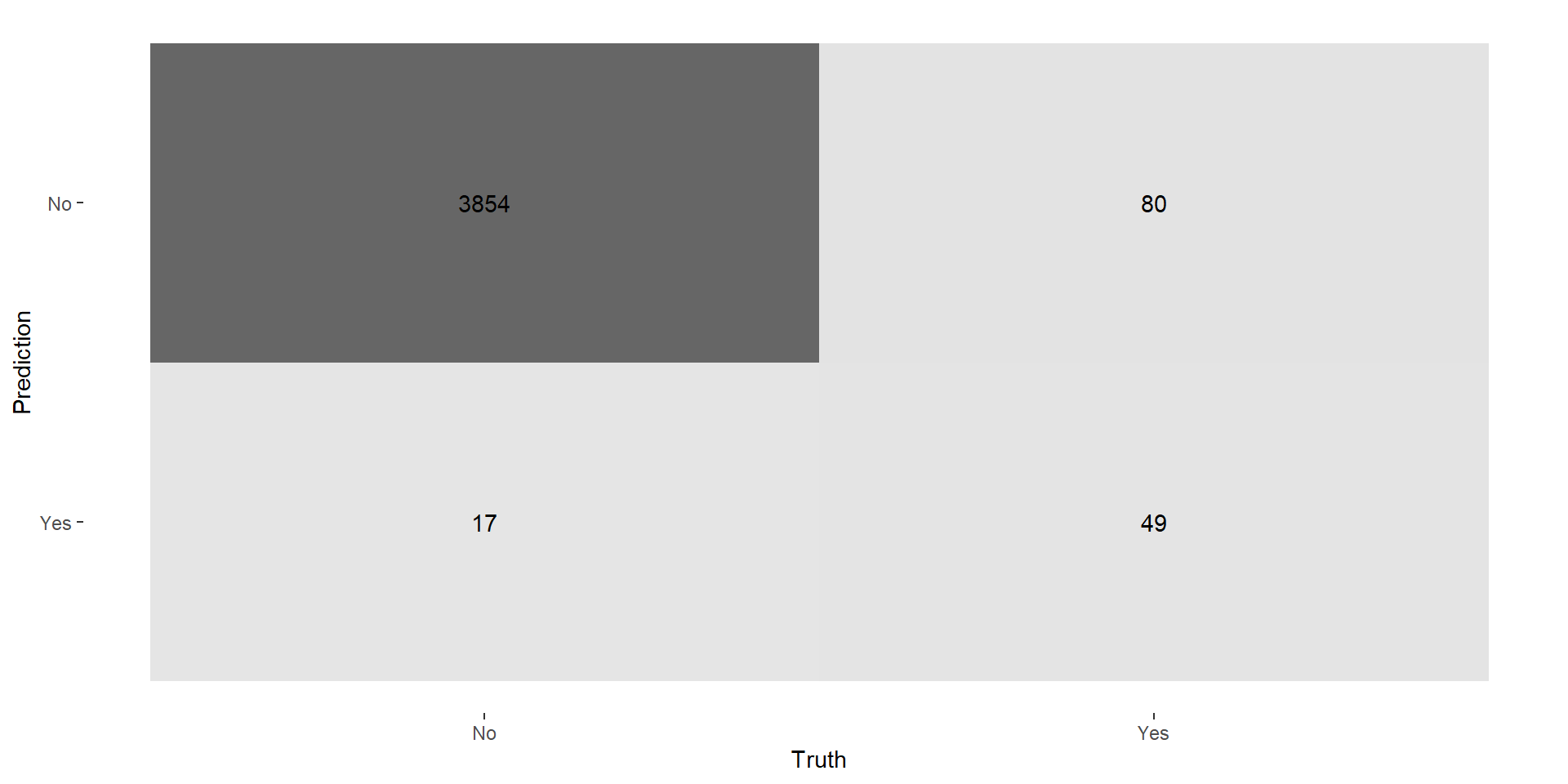
Logistic Regression: Confusion Matrix

default_test_wpreds |>
  conf_mat(truth = default, estimate = logistic_preds) |> 
  autoplot(type = "heatmap")

Classification Metrics

  • Accuracy: proportion of your classes that are correct \[(TP + TN)/Total\]
  • Recall/Sensitivity: proportion of true positives correct (true positive rate) \[TP/(TP+FN)\]
  • Precision/Positive Predictive Value (PPV): proportion of predicted positive that are correct \[TP/(TP+FP)\]
  • Specificity: proportion of true negatives correct (true negative rate) \[TN/(TN+FP)\]
  • Negative Predictive Value (NPV): proportion of predicted negatives that are correct \[TN/(TN+FN)\]

KNN: Performance

default_test_wpreds |>
  conf_mat(truth = default, estimate = knn_preds) |> 
  autoplot("heatmap")

  • Accuracy: \((3854+49)/4000 = .976 = 97.6\%\)
  • Recall/Sensitivity: \(49/(49+80) = 0.380 = 38.0\%\)
  • Precision/Positive Predictive Value (PPV): \(49/(49+17) = .742 = 74.2\%\)
  • Specificity: \(3854/(3854+17) = 0.996 = 99.6\%\)
  • Negative Predictive Value (NPV): \(3854/(3854+80) = 98.0\)

Logistic Regression: Performance

default_test_wpreds |>
  conf_mat(truth = default, estimate = logistic_preds) |> 
  autoplot("heatmap")

Compute the following and write your answers on the board:

  • Accuracy
  • Recall/Sensitivity
  • Precision/Positive Predictive Value (PPV)
  • Specificity
  • Negative Predictive Value (NPV)

Performance Metrics with yardstick

  • yardstick is a package that ships with tidymodels meant for model evaluation
  • Typical syntax: metricname(data, truth, estimate, ...)
    • Bind original data with predicted observations
    • Put true response in for truth and predicted values in for estimate

Logistic Regression: Accuracy

default_test_wpreds |> 
  accuracy(truth = default, estimate = logistic_preds) |> 
  kable()
.metric .estimator .estimate
accuracy binary 0.973

Two More Metrics

  • Matthews correlation coefficient (MCC): similar to \(R^2\) but for classification \[\frac{TP\times TN - FP \times FN}{\sqrt{(TP + FP)(TP+FN)(TN+FP)(TN+FN)}}\]
    • Good for imbalanced data
    • Considers both positives and negatives
  • F-Measure: harmonic mean of recall and precision \[\frac{2}{recall^{-1} + precision^{-1}} = \frac{2TP}{2TP+FP+FN}\]
    • Focuses more on positives
    • bad of imbalanced data

Metric Sets

binary_metrics <- metric_set(accuracy, recall, precision, specificity,
                             npv, mcc, f_meas)
  • Can apply this to compute a bunch of metrics

KNN: Performance

default_test_wpreds |> 
  binary_metrics(truth = default, estimate = knn_preds, event_level = "second") |> 
  kable()
.metric .estimator .estimate
accuracy binary 0.9757500
recall binary 0.3798450
precision binary 0.7424242
specificity binary 0.9956084
npv binary 0.9796645
mcc binary 0.5206828
f_meas binary 0.5025641

Logistic Regression: Performance

default_test_wpreds |> 
  binary_metrics(truth = default, estimate = logistic_preds, event_level = "second") |> 
  kable()
.metric .estimator .estimate
accuracy binary 0.9730000
recall binary 0.3023256
precision binary 0.6842105
specificity binary 0.9953500
npv binary 0.9771747
mcc binary 0.4437097
f_meas binary 0.4193548

Discussion

  • For each of the following metrics, brainstorm a situation in which that metric is probably the most important:
    • Recall
    • Precision
    • Accuracy