MATH 427: ROC Curve and AUC

Eric Friedlander

Announcements

On March 5th at 10am in JAAC, Kyle Mayer will be guest lecturing to talk about his role as a data analyst at Micron. Kyle has a Bachelors in Engineering and a Masters in Physics.

Bio: Kyle Mayer is a Senior Data Analytics Engineer at Micron Technology with over 15 years of experience. He currently supports the Global Quality organization with engineering and data science projects. Kyle specializes in modeling complex physical processes, delivering insights that drive business value. Leveraging his expertise in semiconductor manufacturing, Kyle has developed tools and processes that have prevented over $100M in lost revenue. His passion for applying artificial intelligence to solve complex problems and develop automated systems highlights his commitment to innovation. In his spare time, Kyle enjoys spending time with his kids and going on hikes.

Job Application 1

• Job Ad
• Directions and Resources
• Rubic (in progress)
• Due Next Friday: CV and Cover Letter
• Due Friday March 21st: whole application

Computational Set-Up

library(tidyverse)
library(tidymodels)
library(knitr)
library(janitor) # for contingency tables
library(ISLR2)
library(ggforce) # sina plots

tidymodels_prefer()

set.seed(427)

Default Dataset

A simulated data set containing information on ten thousand customers. The aim here is to predict which customers will default on their credit card debt.

head(Default) |> kable()  # print first six observations

default	student	balance	income
No	No	729.5265	44361.625
No	Yes	817.1804	12106.135
No	No	1073.5492	31767.139
No	No	529.2506	35704.494
No	No	785.6559	38463.496
No	Yes	919.5885	7491.559

Response Variable: default

Default |> 
  tabyl(default) |>  # class frequencies
  kable()           # Make it look nice

default	n	percent
No	9667	0.9667
Yes	333	0.0333

Split the data

set.seed(427)

default_split <- initial_split(Default, prop = 0.6, strata = default)
default_split

<Training/Testing/Total>
<6000/4000/10000>

default_train <- training(default_split)
default_test <- testing(default_split)

K-Nearest Neighbors Classifier: Build Model

• Response (\(Y\)): default
• Predictor (\(X\)): balance

knnfit <- nearest_neighbor(neighbors = 10) |> 
  set_engine("kknn") |> 
  set_mode("classification") |>  
  fit(default ~ balance, data = default_train)   # fit 10-nn model

K-Nearest Neighbors Classifier: Predictions

• Class labels
• Probabilities

predict(knnfit, new_data = default_test, type = "class") |> head() |> kable()   # obtain predictions as classes

.pred_class
No
No
No
No
No
No

• Predicts class w/ maximum probability

predict(knnfit, new_data = default_test, type = "prob") |> head() |> kable() # obtain predictions as probabilities

.pred_No	.pred_Yes
1	0
1	0
1	0
1	0
1	0
1	0

Fitting a logistic regression

Fitting a logistic regression model with default as the response and balance as the predictor:

logregfit <- logistic_reg() |> 
  set_engine("glm") |> 
  fit(default ~ balance, data = default_train)   # fit logistic regression model

tidy(logregfit) |> kable()  # obtain results

term	estimate	std.error	statistic	p.value
(Intercept)	-10.6926385	0.4659035	-22.95033	0
balance	0.0055327	0.0002841	19.47329	0

Making predictions in R

• Class Labels
• Log-Odds
• Probabilities

predict(logregfit, new_data = tibble(balance = 700), type = "class") |> kable()   # obtain class predictions

.pred_class
No

predict(logregfit, new_data = tibble(balance = 700), type = "raw") |> kable()   # obtain log-odds predictions

x
-6.819727

predict(logregfit, new_data = tibble(balance = 700), type = "prob") |> kable()  # obtain probability predictions

.pred_No	.pred_Yes
0.9989092	0.0010908

Binary Classifiers

• Start with binary classification scenarios
• With binary classification, designate one category as “Success/Positive” and the other as “Failure/Negative”
  • If relevant to your problem: “Positive” should be the thing you’re trying to predict/care more about
  • Note: “Positive” \(\neq\) “Good”
  • For default: “Yes” is Positive
• Some metrics weight “Positives” more and viceversa

Last Time

• Confusion Matrix
• Metrics based on confusion matrix
  • Accuracy
  • Recall/Sensitivity
  • Precision/PPV
  • Specificity
  • NPV
  • MCC
  • F-Measure
• Today: ROC and AUC

Thresholding

Using a threshold

• Step 1: Predict probabilities for all observations

default_test_wprobs <- default_test |>
  mutate(
    knn_probs = predict(knnfit, new_data = default_test, type = "prob") |> pull(.pred_Yes),
    logistic_probs = predict(logregfit, new_data = default_test, type = "prob") |> pull(.pred_Yes)
  )

default_test_wprobs |> head() |> kable()   # obtain probability predictions

default	student	balance	income	knn_probs	logistic_probs
No	No	729.5265	44361.63	0	0.0012842
No	Yes	808.6675	17600.45	0	0.0019883
No	Yes	1220.5838	13268.56	0	0.0190870
No	No	237.0451	28251.70	0	0.0000843
No	No	606.7423	44994.56	0	0.0006514
No	No	286.2326	45042.41	0	0.0001107

Using a threshold

• Step 1: Predict probabilities for all observations
• Step 2: Set a threshold to obtain class labels (0.5 below)

threshold <- 0.5   # set threshold
default_test_wprobs <- default_test_wprobs |>
  mutate(knn_preds = as_factor(if_else(knn_probs > threshold, "Yes", "No")),
         logistic_preds = as_factor(if_else(logistic_probs > threshold, "Yes", "No"))
  )

default_test_wprobs |> head() |> kable()

default	student	balance	income	knn_probs	logistic_probs	knn_preds	logistic_preds
No	No	729.5265	44361.63	0	0.0012842	No	No
No	Yes	808.6675	17600.45	0	0.0019883	No	No
No	Yes	1220.5838	13268.56	0	0.0190870	No	No
No	No	237.0451	28251.70	0	0.0000843	No	No
No	No	606.7423	44994.56	0	0.0006514	No	No
No	No	286.2326	45042.41	0	0.0001107	No	No

Using a threshold

• Step 1: Predict probabilities for all observations
• Step 2: Set a threshold to obtain class labels (0.5 below)

threshold <- 0.5   # set threshold
default_test_wprobs <- default_test_wprobs |>
  mutate(knn_preds = as_factor(if_else(knn_probs > threshold, "Yes", "No")),
         logistic_preds = as_factor(if_else(logistic_probs > threshold, "Yes", "No")))

default_test_wprobs |> head() |> kable()

default	student	balance	income	knn_probs	logistic_probs	knn_preds	logistic_preds
No	No	729.5265	44361.63	0	0.0012842	No	No
No	Yes	808.6675	17600.45	0	0.0019883	No	No
No	Yes	1220.5838	13268.56	0	0.0190870	No	No
No	No	237.0451	28251.70	0	0.0000843	No	No
No	No	606.7423	44994.56	0	0.0006514	No	No
No	No	286.2326	45042.41	0	0.0001107	No	No

Performance

roc_metrics <- metric_set(accuracy, sensitivity, specificity)
roc_metrics(default_test_wprobs, truth = default, estimate = knn_preds, event_level = "second") |> kable()

.metric	.estimator	.estimate
accuracy	binary	0.9717500
sensitivity	binary	0.3565891
specificity	binary	0.9922501

Low Threshold

threshold <- 0.1   # set threshold
default_test_wprobs <- default_test_wprobs |>
  mutate(knn_preds = as_factor(if_else(knn_probs > threshold, "Yes", "No")))

roc_metrics(default_test_wprobs, truth = default, estimate = knn_preds, event_level = "second")  |> kable()

.metric	.estimator	.estimate
accuracy	binary	0.9060000
sensitivity	binary	0.7364341
specificity	binary	0.9116507

High Threshold

threshold <- 0.9   # set threshold
default_test_wprobs <- default_test_wprobs |>
  mutate(knn_preds = as_factor(if_else(knn_probs > threshold, "Yes", "No"))
  )

roc_metrics(default_test_wprobs, truth = default, estimate = knn_preds, event_level = "second") |> kable()

.metric	.estimator	.estimate
accuracy	binary	0.9685000
sensitivity	binary	0.0310078
specificity	binary	0.9997417

Question

• If I want to improve Recall/Sensitivity should I increase or decrease my threshold?
• If I want to improve my Precision/PPV should I increase or decrease my threshold?

ROC Curve

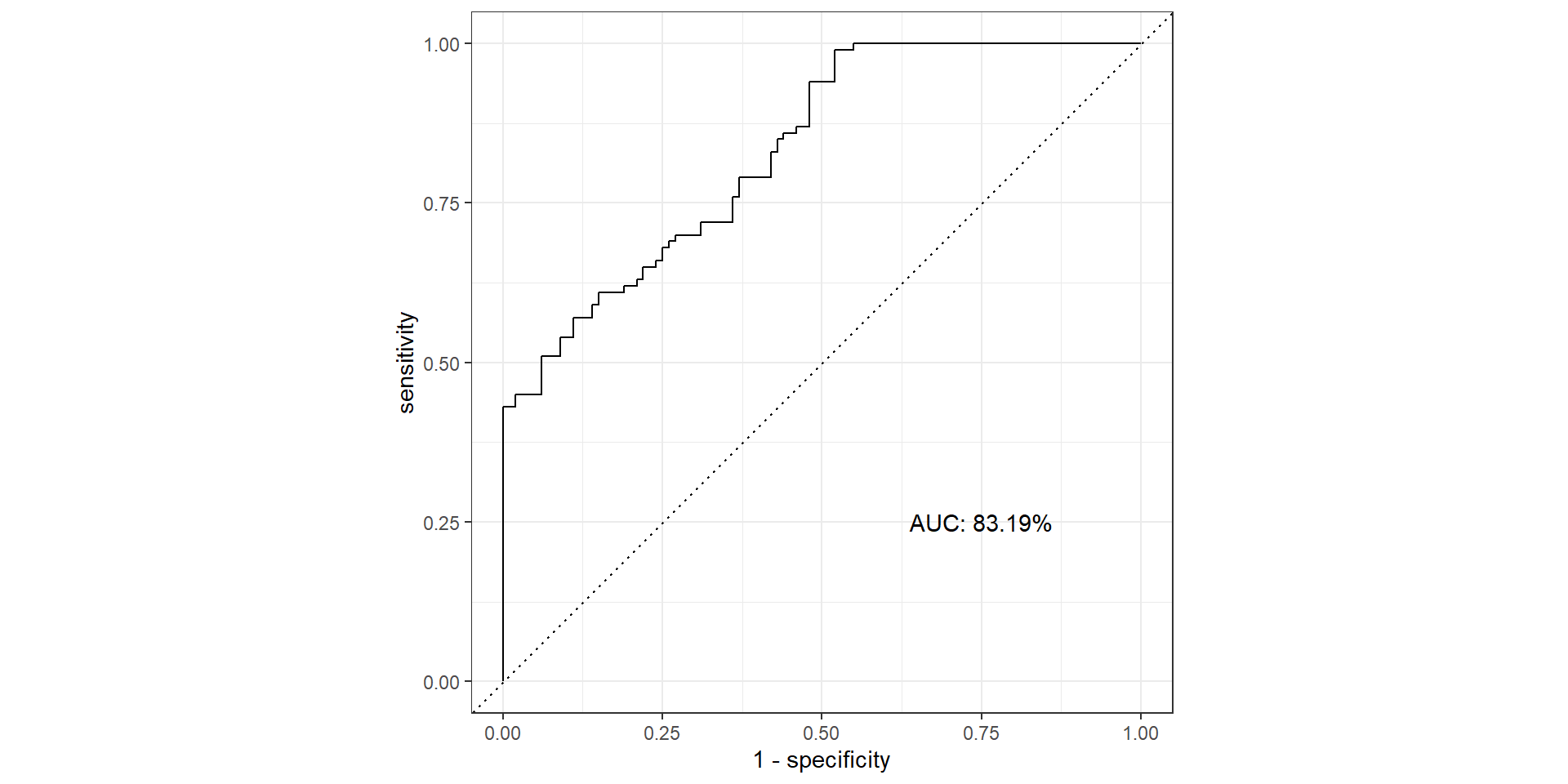
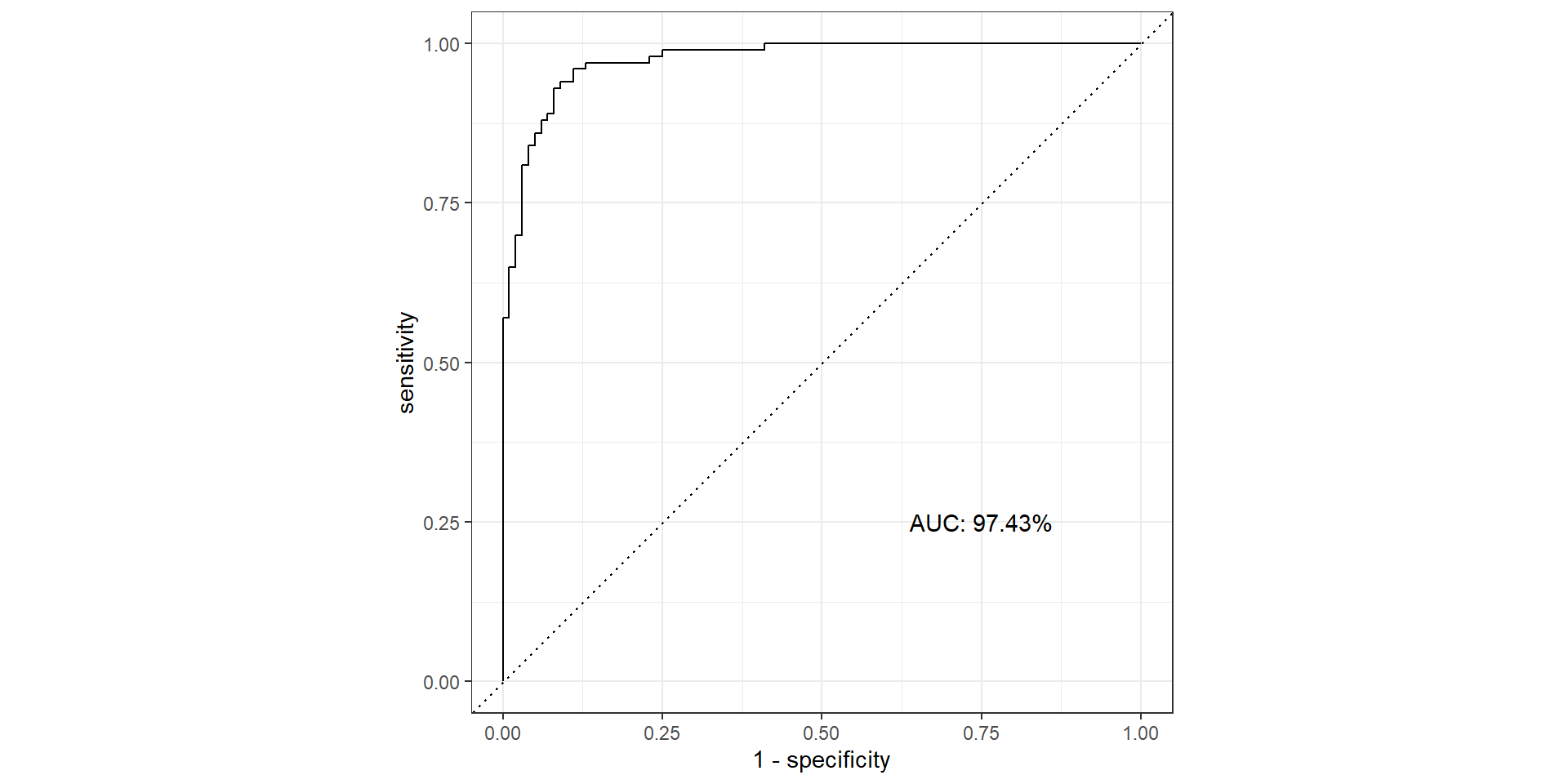
ROC Curve and AUC

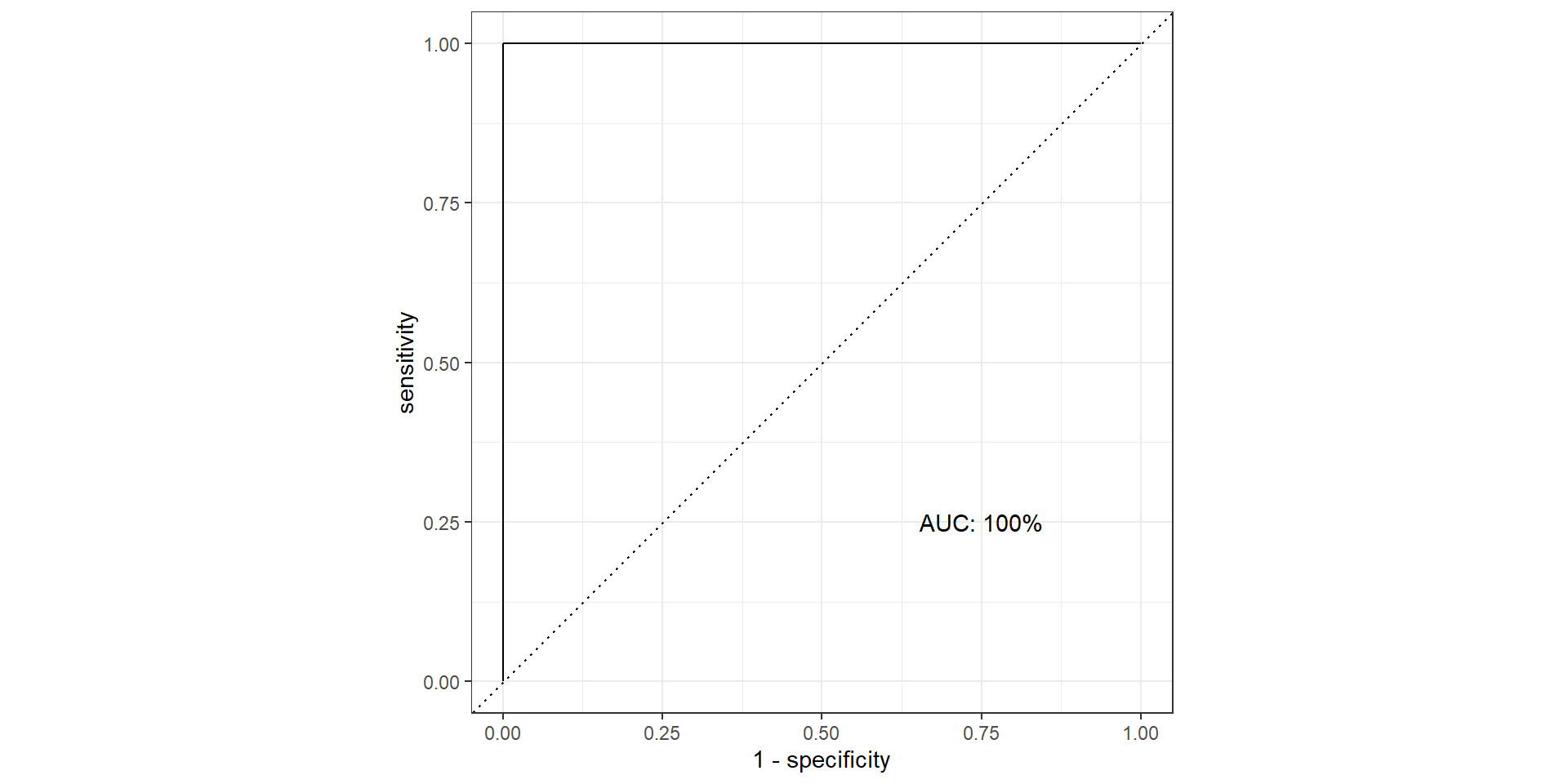
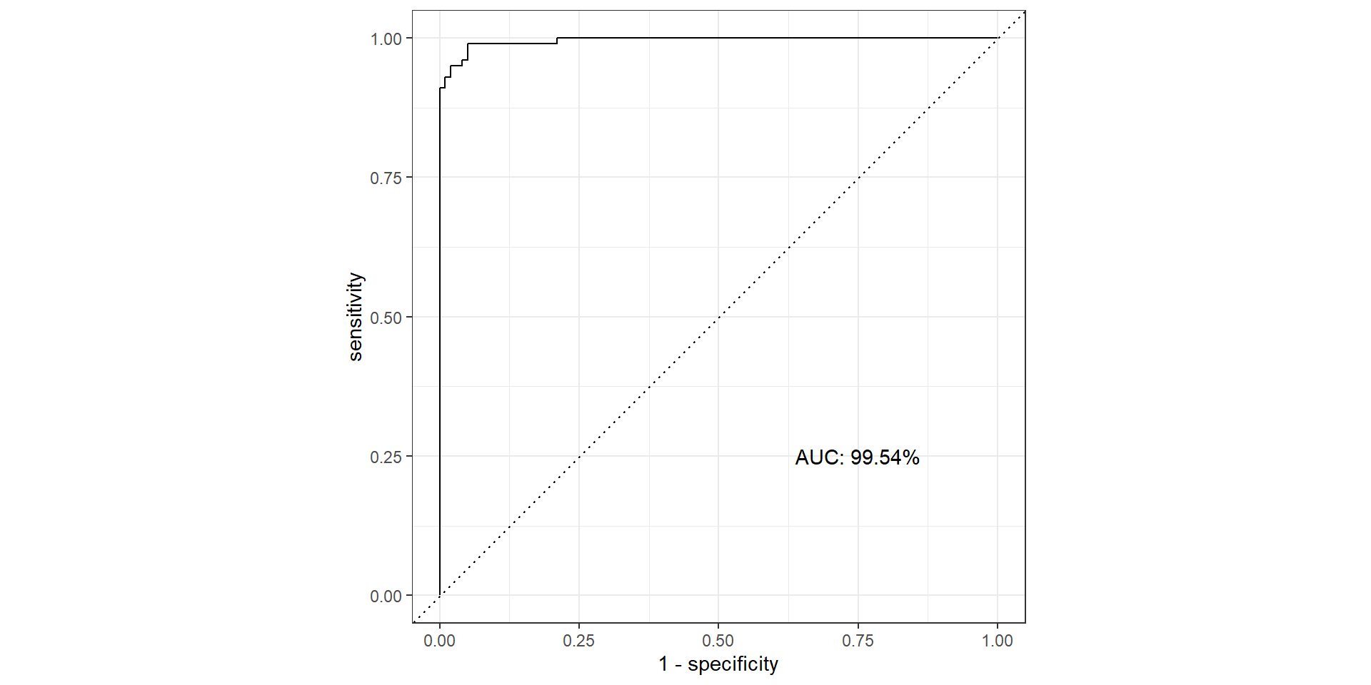
• ROC (Receiver Operating Characteristics) curve: popular graphic for comparing different classifiers across all possible thresholds
  • Plots the (1-Specificity) along the x-axis and the Sensitivity (true positive rate) along the y-axis
• AUC: area under the AUC curve
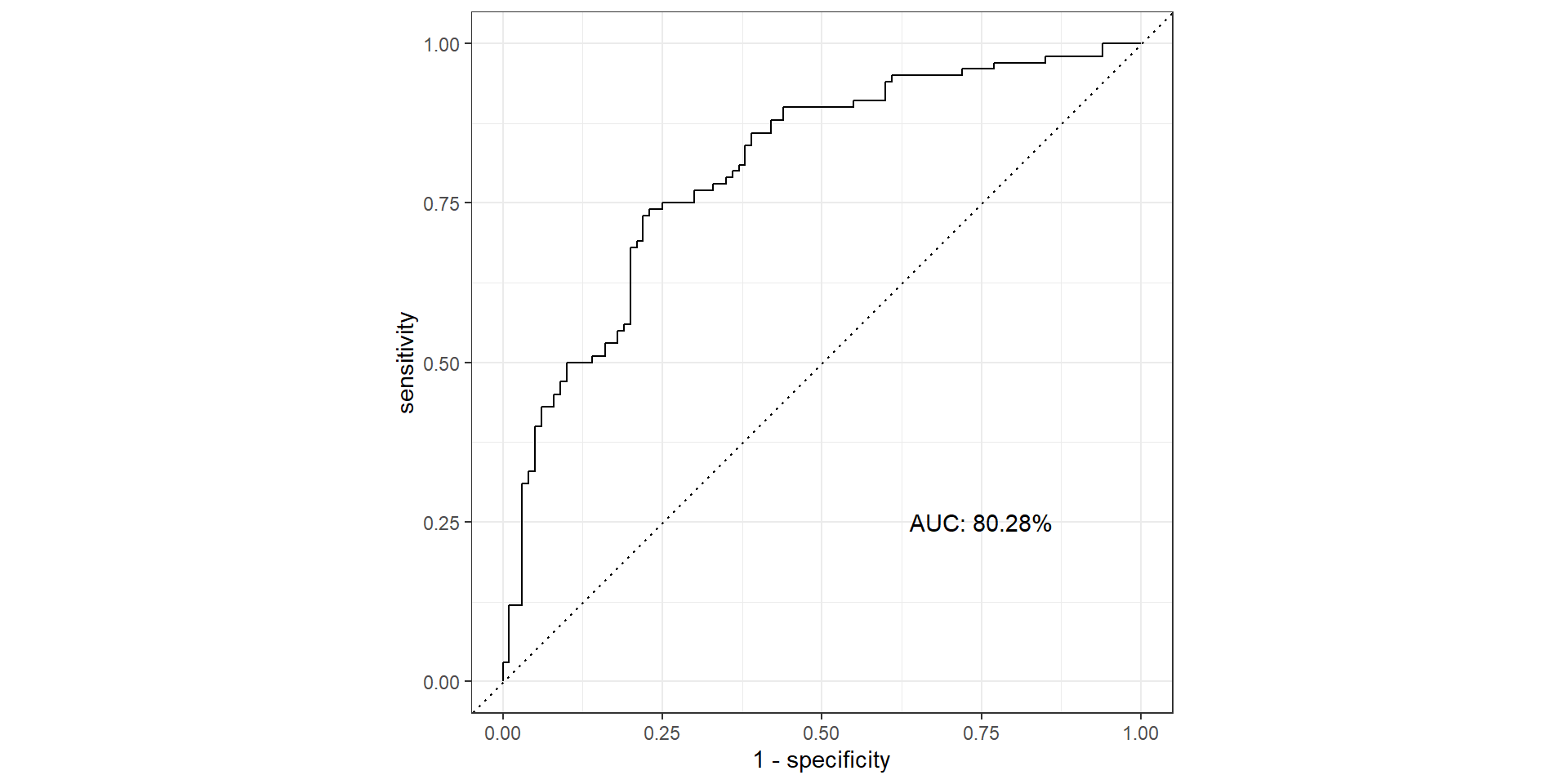
  • Ideal ROC curve will hug the top left corner
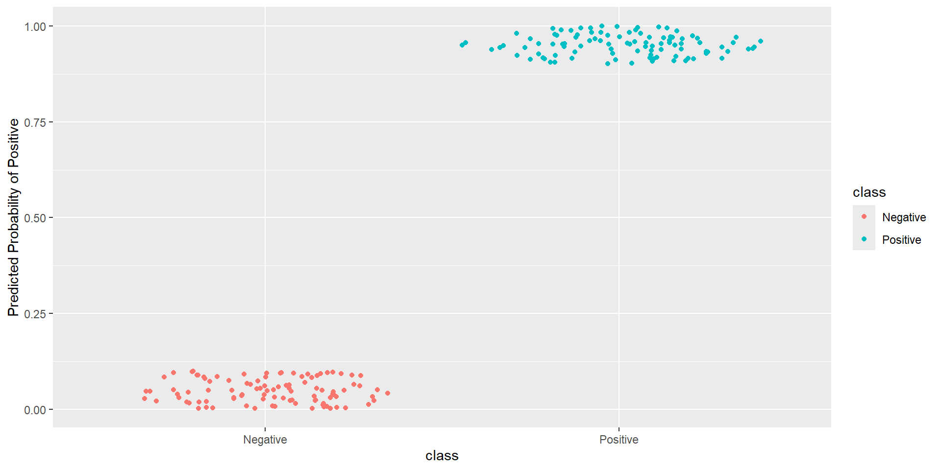
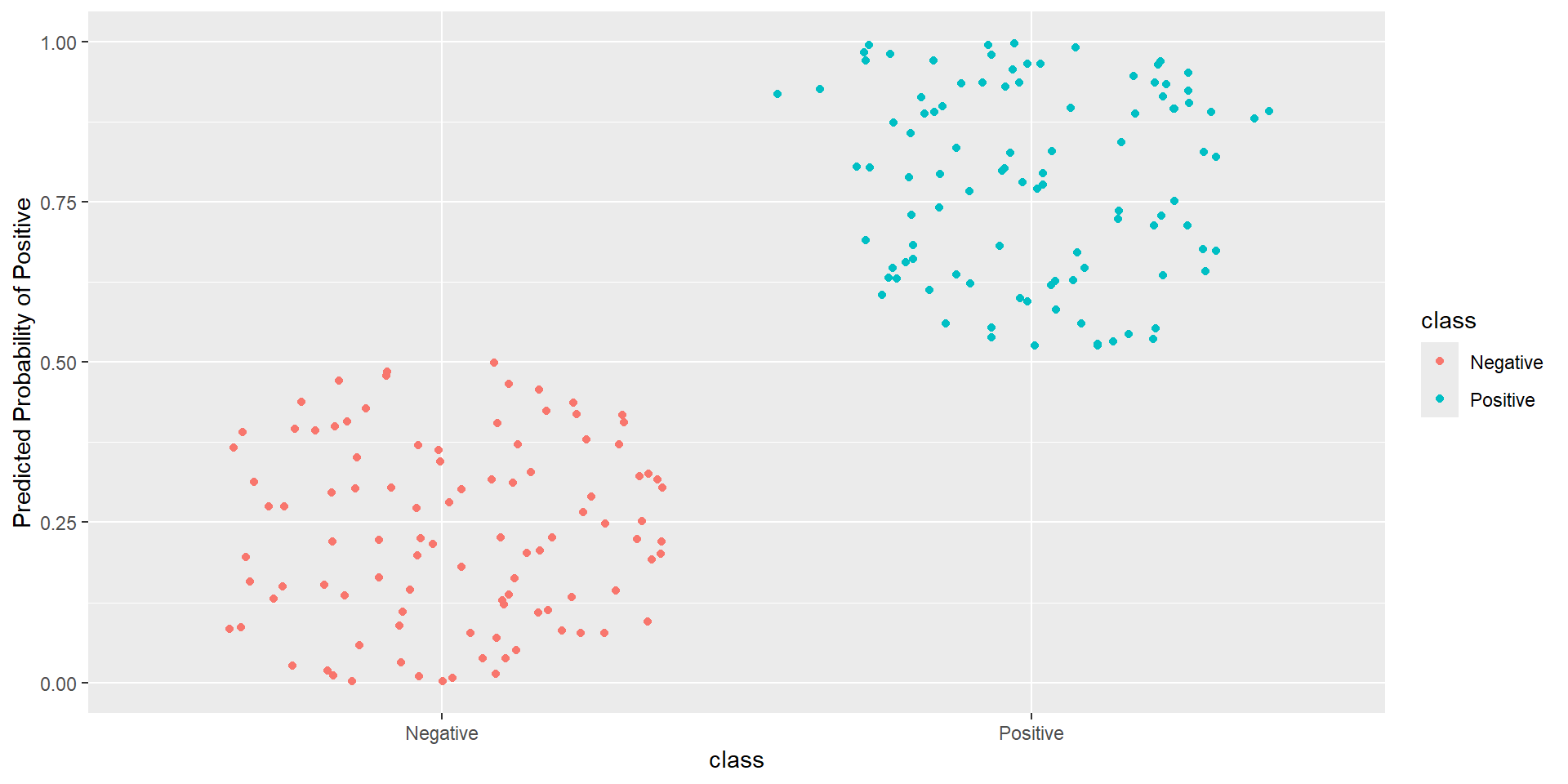
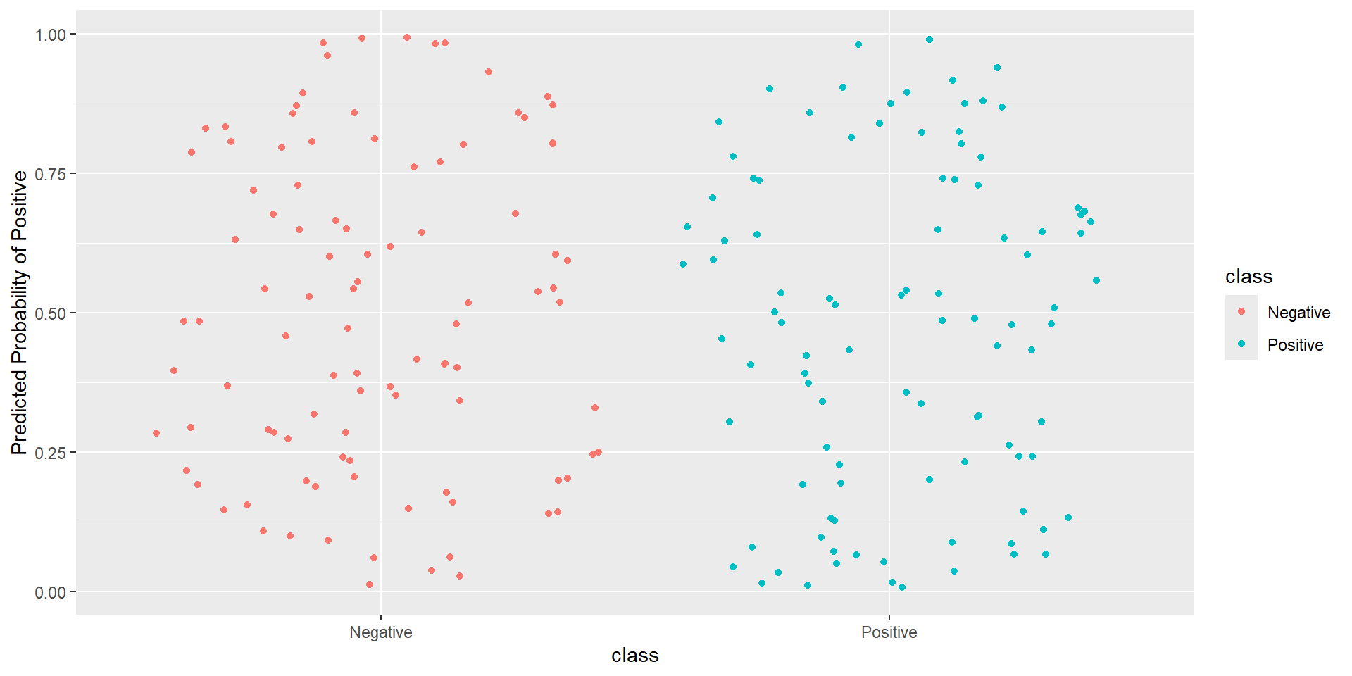
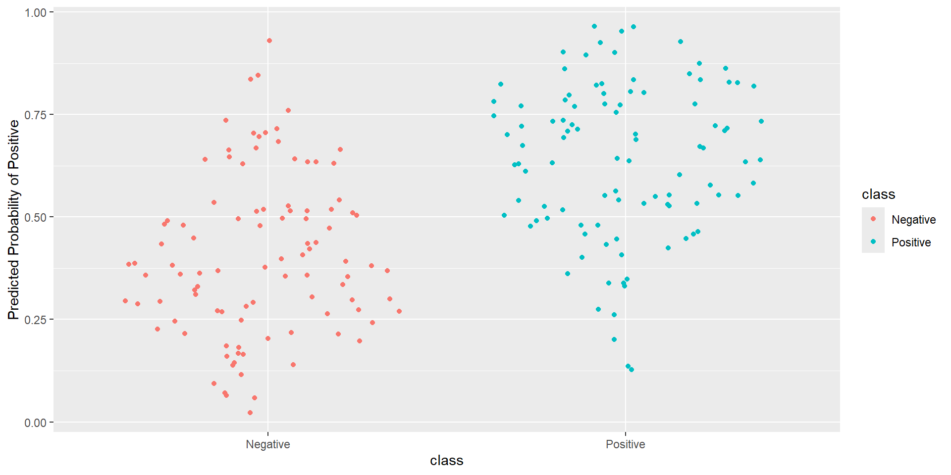
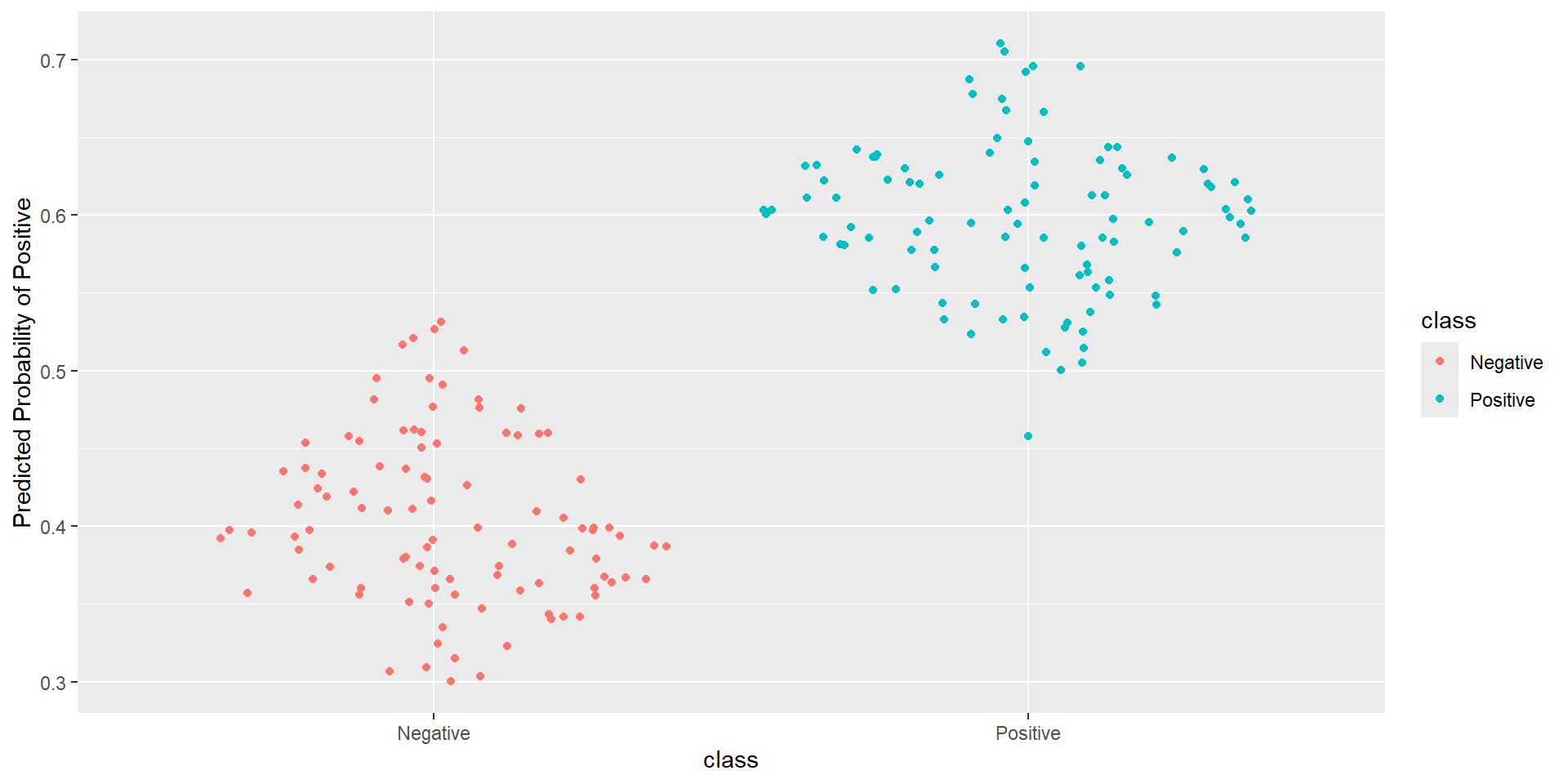
• Idea: How well is my classifier separating positives from negatives

ROC Curve

roc_curve(default_test_wprobs, truth = default, knn_probs, event_level = "second") |>
  head() |>
  kable()

.threshold	specificity	sensitivity
-Inf	0.0000000	1.0000000
0.0000	0.0000000	1.0000000
0.0145	0.8796177	0.8217054
0.0415	0.8858176	0.8139535
0.0560	0.8971842	0.7829457
0.0655	0.8979592	0.7751938

ROC Curve: Plot

roc_curve(default_test_wprobs, truth = default, knn_probs, event_level = "second") |>
  autoplot()

AUC

• AUC: Area under the curve (ROC Curve that is)
• Measures how good your model is at separating categories
• Only for binary classification

AUC in R

roc_auc(default_test_wprobs, truth = default, knn_probs, event_level = "second") |>
  kable()

.metric	.estimator	.estimate
roc_auc	binary	0.8757397

Pathological Example 1

Pathological Example 2

Pathological Example 3

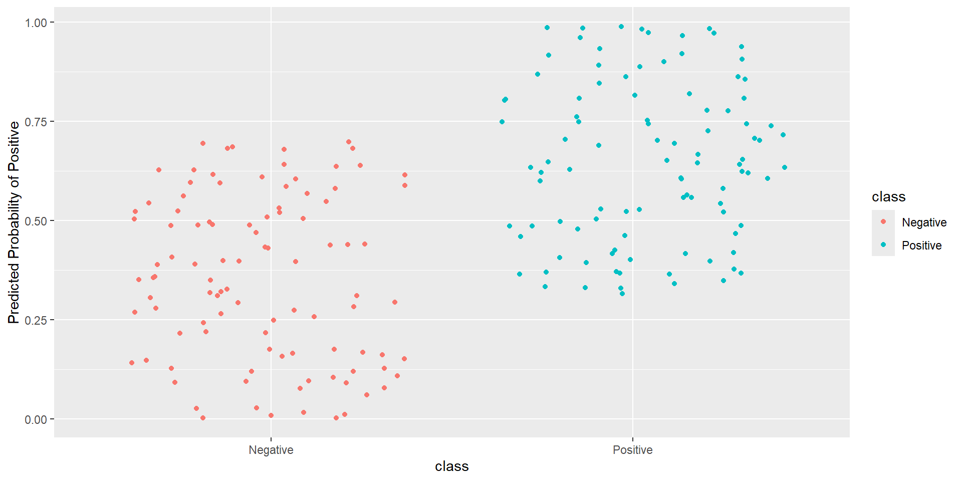
Pathological Example 4

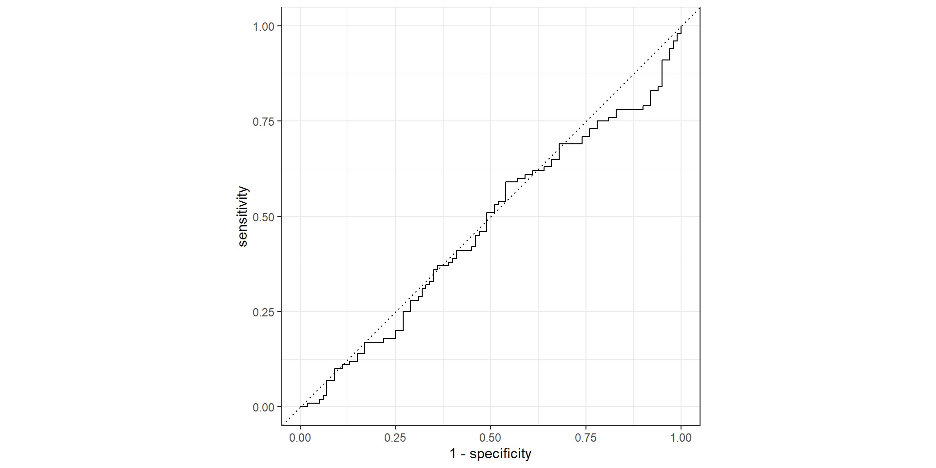
Pathological Example 5

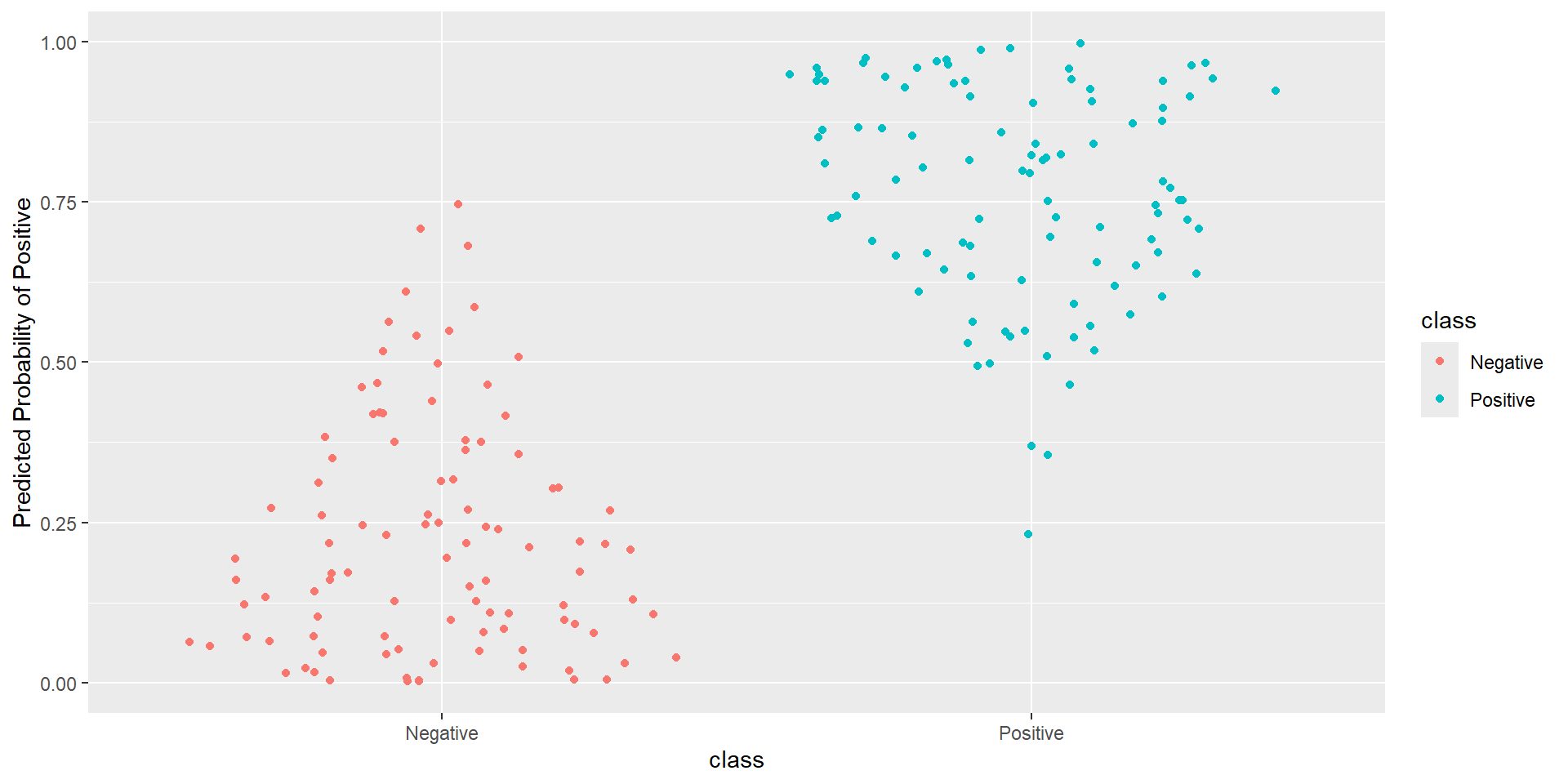
Pathological Example 6

Pathological Example 7

AUC Questions

• What should be the minimum AUC?
• What should be that maximum possible AUC?