MATH 427: Preprocessing, Missing Data, and Resampling Continued

Eric Friedlander

Announcements

Coyote Connections Thu March 13th 7-9pm
Please print out and bring four copies of your resume and cover letter to class on Friday
Debrief from talk today

Computational Set-Up

library(tidyverse)
library(tidymodels)
library(knitr)
library(janitor) # for contingency tables
library(ISLR2)
library(readODS)

tidymodels_prefer()

set.seed(427)

Pre-processing

Data: Different Ames Housing Prices

Goal: Predict Sale_Price.

ames <- read_rds("../data/AmesHousing.rds")
ames |> glimpse()

Rows: 881
Columns: 20
$ Sale_Price    <int> 244000, 213500, 185000, 394432, 190000, 149000, 149900, …
$ Gr_Liv_Area   <int> 2110, 1338, 1187, 1856, 1844, NA, NA, 1069, 1940, 1544, …
$ Garage_Type   <fct> Attchd, Attchd, Attchd, Attchd, Attchd, Attchd, Attchd, …
$ Garage_Cars   <dbl> 2, 2, 2, 3, 2, 2, 2, 2, 3, 3, 2, 3, 3, 2, 2, 2, 3, 2, 2,…
$ Garage_Area   <dbl> 522, 582, 420, 834, 546, 480, 500, 440, 606, 868, 532, 7…
$ Street        <fct> Pave, Pave, Pave, Pave, Pave, Pave, Pave, Pave, Pave, Pa…
$ Utilities     <fct> AllPub, AllPub, AllPub, AllPub, AllPub, AllPub, AllPub, …
$ Pool_Area     <int> 0, 0, 0, 0, 0, 0, 0, 0, 0, 0, 0, 0, 0, 0, 0, 0, 0, 0, 0,…
$ Neighborhood  <fct> North_Ames, Stone_Brook, Gilbert, Stone_Brook, Northwest…
$ Screen_Porch  <int> 0, 0, 0, 0, 0, 0, 0, 165, 0, 0, 0, 0, 0, 0, 0, 0, 0, 0, …
$ Overall_Qual  <fct> Good, Very_Good, Above_Average, Excellent, Above_Average…
$ Lot_Area      <int> 11160, 4920, 7980, 11394, 11751, 11241, 12537, 4043, 101…
$ Lot_Frontage  <dbl> 93, 41, 0, 88, 105, 0, 0, 53, 83, 94, 95, 90, 105, 61, 6…
$ MS_SubClass   <fct> One_Story_1946_and_Newer_All_Styles, One_Story_PUD_1946_…
$ Misc_Val      <int> 0, 0, 500, 0, 0, 700, 0, 0, 0, 0, 0, 0, 0, 0, 0, 0, 0, 0…
$ Open_Porch_SF <int> 0, 0, 21, 0, 122, 0, 0, 55, 95, 35, 70, 74, 130, 82, 48,…
$ TotRms_AbvGrd <int> 8, 6, 6, 8, 7, 5, 6, 4, 8, 7, 7, 7, 7, 6, 7, 7, 10, 7, 7…
$ First_Flr_SF  <int> 2110, 1338, 1187, 1856, 1844, 1004, 1078, 1069, 1940, 15…
$ Second_Flr_SF <int> 0, 0, 0, 0, 0, 0, 0, 0, 0, 0, 0, 0, 563, 0, 886, 656, 11…
$ Year_Built    <int> 1968, 2001, 1992, 2010, 1977, 1970, 1971, 1977, 2009, 20…

Today

Well cover some common pre-processing tasks:

Dealing with zero-variance (zv) and/or near-zero variance (nzv) variables
Imputing missing entries
Label encoding ordinal categorical variables
Standardizing (centering and scaling) numeric predictors
Lumping predictors
One-hot/dummy encoding categorical predictor

Pre-Split Cleaning

Before you split your data: make sure data is in correct format
This may mean different things for different data sets
Common examples:
- Fixing names of columns
- Ensure all variable types are correct
- Ensure all factor levels are correct and in order (if applicable)
- Remove any variables that are not important (or harmful) to your analysis
- Ensure missing values are coded as such (i.e. as NA instead of 0 or -1 or “missing”)
- Filling in missing values where you know what the answer should be (i.e. if a missing value really means 0 instead of missing)

Example: Factor Levels in Wrong Order

ames |> pull(Overall_Qual) |> levels()

 [1] "Above_Average"  "Average"        "Below_Average"  "Excellent"     
 [5] "Fair"           "Good"           "Poor"           "Very_Excellent"
 [9] "Very_Good"      "Very_Poor"

Re-Factoring

ames <- ames |> 
  mutate(Overall_Qual = factor(Overall_Qual, levels = c("Very_Poor", "Poor", 
                                                        "Fair", "Below_Average",
                                                        "Average", "Above_Average", 
                                                        "Good", "Very_Good",
                                                        "Excellent", "Very_Excellent")))
ames |> pull(Overall_Qual) |> levels()

 [1] "Very_Poor"      "Poor"           "Fair"           "Below_Average" 
 [5] "Average"        "Above_Average"  "Good"           "Very_Good"     
 [9] "Excellent"      "Very_Excellent"

Zero-Variance (zv) and/or Near-Zero Variance (nzv) Variables

Heuristic for detecting near-zero variance features is:

The fraction of unique values over the sample size is low (say ≤ 10%).
The ratio of the frequency of the most prevalent value to the frequency of the second most prevalent value is large (say ≥ 20%).

library(caret)
nearZeroVar(ames, saveMetrics = TRUE) |> kable()

	freqRatio	percentUnique	zeroVar	nzv
Sale_Price	1.000000	55.7321226	FALSE	FALSE
Gr_Liv_Area	1.333333	62.9965948	FALSE	FALSE
Garage_Type	2.196581	0.6810443	FALSE	FALSE
Garage_Cars	1.970213	0.5675369	FALSE	FALSE
Garage_Area	2.250000	38.0249716	FALSE	FALSE
Street	219.250000	0.2270148	FALSE	TRUE
Utilities	880.000000	0.2270148	FALSE	TRUE
Pool_Area	876.000000	0.6810443	FALSE	TRUE
Neighborhood	1.476744	2.9511918	FALSE	FALSE
Screen_Porch	199.750000	6.6969353	FALSE	TRUE
Overall_Qual	1.119816	1.1350738	FALSE	FALSE
Lot_Area	1.071429	79.7956867	FALSE	FALSE
Lot_Frontage	1.617021	11.5777526	FALSE	FALSE
MS_SubClass	1.959064	1.7026107	FALSE	FALSE
Misc_Val	141.833333	1.9296254	FALSE	TRUE
Open_Porch_SF	23.176471	19.2962543	FALSE	FALSE
TotRms_AbvGrd	1.311225	1.2485812	FALSE	FALSE
First_Flr_SF	1.777778	63.7911464	FALSE	FALSE
Second_Flr_SF	64.250000	31.3280363	FALSE	FALSE
Year_Built	1.125000	12.0317821	FALSE	FALSE

Recipe: Near-Zero Variance

preproc <- recipe(Sale_Price ~ ., data = ames) |> 
  step_nzv(all_predictors()) # remove zero or near-zero variable predictors

Missing Data

Many times, you can’t just drop missing data
Even if you can, dropping missing values can generate biased data/models
Sometimes missing data gives you more information
Types of missing data:
- Missing completely at random (MCAR): there is no pattern to your missing values
- Missing at random (MAR): missing values are dependent on other values in the data set
- Missing not at random (MNAR): missing values are dependent on the value that is missing
Structured missingness (SM): when the missingness of certain values are depends on one another, regardless of whether the missing values are MCAR, MAR, or MNAR

MCAR: Examples

Sensor data: occasionally sensors break so you’re missing data randomly
Survey data: sometimes people just randomly skip questions
Survey data: customers are randomly given 5 questions from a bank of 100 questions

MAR: Examples

Men are less likely to respond to surveys about depression
Medical study: patients who miss follow-up appointments are more likely to be young
Survey responses: ESL respondents may be more likely to skip certain questions that are difficult to interpret (only MAR if you know they are ESL)
Measure of student performance: students who score lower are more likely to skip questions

MNAR: Examples

Survey on income: respondent may be less likely to report their income if they are poor
Survey about political beliefs: respondent may be more likely to skip questions when their answer is perceived as undesirable
Customer satisfaction: only customers who feel strongly respond
Medical study: patients refuse to report unhealthy habits

Structurally Missing: Examples

Health survey: all questions related to pregnancy are left blank by males
Bank data set: combination of home, auto, and credit cards… not all customer have all three so have missing data in certain portions
Survey: many respondents by stop the survey early so all questions after a certain point are missing
Netflix: customers may only watch similar movies and TV shows

Remedies for Missing Data

Lot of complicated ways that you can read about
Can drop column of too much of the data is missing
Imputing:
- step_impute_median: used for numeric (especially discrete) variables
- step_impute_mean: used for numeric variables
- step_impute_knn: used for both numeric and categorical variables (computationally expensive)
- step_impute_mode: used for nominal (having no order) categorical variable

Exploring Missing Data

ames |> 
  summarize(across(everything(), ~ sum(is.na(.)))) |> 
  pivot_longer(everything()) |> 
  filter(value > 0) |> 
  kable()

name	value
Gr_Liv_Area	113
Garage_Type	54
Year_Built	41

Missing Data: Garage_Type

The reason that Garage_Type is missing is because there is no basement
- Solution: replace NAs with No_Garage
- Do this before data splitting

Fixing Garage_Type

ames <- ames |> 
  mutate(Garage_Type = as_factor(if_else(is.na(Garage_Type), "No_Garage", Garage_Type)))

Missing Data: Year_Built

MCAR
- Solution 1: Impute with mean or median
- Solution 2: Impute with KNN… maybe we can infer what the values are based on other values in the data set?

Missing Data: Gr_Liv_Area

MCAR
- Solution 1: Impute with mean or median
- Solution 2: Impute with KNN… maybe we can infer what the values are based on other values in the data set?

Recipe: Missing Data

preproc <- recipe(Sale_Price ~ ., data = ames) |> 
  step_nzv(all_predictors()) |>  # remove zero or near-zero variable predictors
  step_impute_knn(Year_Built, Gr_Liv_Area) # impute missing values in Overall_Qual and Year_Built

Note: step_imput_knn uses the “Gower’s Distance” so don’t need to worry about normalizing

Encoding Ordinal Features

Two types of categorical features:

Ordinal (order is important)
Nominal (order is not important)

Encoding Ordinal Features

ames |> pull(Overall_Qual) |> levels()

 [1] "Very_Poor"      "Poor"           "Fair"           "Below_Average" 
 [5] "Average"        "Above_Average"  "Good"           "Very_Good"     
 [9] "Excellent"      "Very_Excellent"

Very_Poor = 1, Poor = 2, Fair = 3, etc…

Recipe: Encoding Ordinal Features

preproc <- recipe(Sale_Price ~ ., data = ames) |> 
  step_nzv(all_predictors()) |>  # remove zero or near-zero variable predictors
  step_impute_knn(Year_Built, Gr_Liv_Area) |>  # impute missing values in Overall_Qual and Year_Built
  step_integer(Overall_Qual) # convert Overall_Qual into ordinal encoding

Lump Small Categories Together

ames |> count(Neighborhood) |> kable()

Neighborhood	n
North_Ames	127
College_Creek	86
Old_Town	83
Edwards	49
Somerset	50
Northridge_Heights	52
Gilbert	47
Sawyer	49
Northwest_Ames	41
Sawyer_West	31
Mitchell	33
Brookside	33
Crawford	22
Iowa_DOT_and_Rail_Road	28
Timberland	21
Northridge	22
Stone_Brook	17
South_and_West_of_Iowa_State_University	21
Clear_Creek	16
Meadow_Village	14
Briardale	10
Bloomington_Heights	10
Veenker	9
Northpark_Villa	3
Blueste	3
Greens	4

Lump Small Categories Together

ames |> mutate(Neighborhood = fct_lump_prop(Neighborhood, 0.05)) |> 
  count(Neighborhood) |>  kable()

Neighborhood	n
North_Ames	127
College_Creek	86
Old_Town	83
Edwards	49
Somerset	50
Northridge_Heights	52
Gilbert	47
Sawyer	49
Other	338

Recipe: Lumping Small Factors Together

preproc <- recipe(Sale_Price ~ ., data = ames) |> 
  step_nzv(all_predictors()) |>  # remove zero or near-zero variable predictors
  step_impute_knn(Year_Built, Gr_Liv_Area) |>  # impute missing values in Overall_Qual and Year_Built
  step_integer(Overall_Qual) |> # convert Overall_Qual into ordinal encoding
  step_other(Neighborhood, threshold = 0.01, other = "Other") # lump all categories with less than 1% representation into a category called Other for each variable

One-hot/dummy encoding categorical predictors

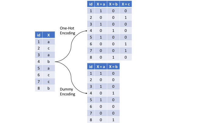
Figure 3.9: Machine Learning with R

Recipe: Dummy Variables

preproc <- recipe(Sale_Price ~ ., data = ames) |> 
  step_nzv(all_predictors()) |>  # remove zero or near-zero variable predictors
  step_impute_knn(Year_Built, Gr_Liv_Area) |>  # impute missing values in Overall_Qual and Year_Built
  step_integer(Overall_Qual) |> # convert Overall_Qual into ordinal encoding
  step_other(Neighborhood, threshold = 0.01, other = "Other") |> # lump all categories with less than 1% representation into a category called Other for each variable
  step_dummy(all_nominal_predictors(), one_hot = TRUE)  # in general use one_hot unless doing linear regression

Recipe: Center and scale

preproc <- recipe(Sale_Price ~ ., data = ames) |> 
  step_nzv(all_predictors()) |>  # remove zero or near-zero variable predictors
  step_impute_knn(Year_Built, Gr_Liv_Area) |>  # impute missing values in Overall_Qual and Year_Built
  step_integer(Overall_Qual) |> # convert Overall_Qual into ordinal encoding
  step_other(Neighborhood, threshold = 0.01, other = "Other") |> # lump all categories with less than 1% representation into a category called Other for each variable
  step_dummy(all_nominal_predictors(), one_hot = TRUE) |>  # in general use one_hot unless doing linear regression
  step_normalize(all_numeric_predictors())

Order of Preprocessing Step

Questions to ask:

Should this be done before or after data splitting?
If I do step_A first what is the impact on step_B? For example, do you want to encode categorical variables before or after normalizing?
What data format is required by the model I’m fitting and how will my model react to these changes?
Is this step part of my “model”? I.e. is this a decision I’m making based on the data or based on subject matter expertise?
Do I have access to my test predictors?

Questions

Should I lump before or after dummy coding?
Should I dummy code before or after normalizing?
Should I lump before my initial split?
How does ordinal encoding impact linear regression vs. KNN?

Final R Workflow

Clean Data Set

ames <- ames |> 
  mutate(Overall_Qual = factor(Overall_Qual, levels = c("Very_Poor", "Poor", 
                                                        "Fair", "Below_Average",
                                                        "Average", "Above_Average", 
                                                        "Good", "Very_Good",
                                                        "Excellent", "Very_Excellent")),
         Garage_Type = if_else(is.na(Garage_Type), "No_Garage", Garage_Type),
         Garage_Type = as_factor(Garage_Type)
         )

Initial Data Split

set.seed(427)

data_split <- initial_split(ames, strata = "Sale_Price")
ames_train <- training(data_split)
ames_test  <- testing(data_split)

Define Folds

ames_folds <- vfold_cv(ames_train, v = 10, repeats = 10)
ames_folds

#  10-fold cross-validation repeated 10 times 
# A tibble: 100 × 3
   splits           id       id2   
   <list>           <chr>    <chr> 
 1 <split [594/66]> Repeat01 Fold01
 2 <split [594/66]> Repeat01 Fold02
 3 <split [594/66]> Repeat01 Fold03
 4 <split [594/66]> Repeat01 Fold04
 5 <split [594/66]> Repeat01 Fold05
 6 <split [594/66]> Repeat01 Fold06
 7 <split [594/66]> Repeat01 Fold07
 8 <split [594/66]> Repeat01 Fold08
 9 <split [594/66]> Repeat01 Fold09
10 <split [594/66]> Repeat01 Fold10
# ℹ 90 more rows

Define Model(s)

lm_model <- linear_reg() |>
  set_engine('lm')

knn5_model <- nearest_neighbor(neighbors = 5) |>
  set_engine("kknn") |>
  set_mode("regression")

knn10_model <- nearest_neighbor(neighbors = 10) |>
  set_engine("kknn") |>
  set_mode("regression")

Define Preprocessing: Linear regression

lm_preproc <- recipe(Sale_Price ~ ., data = ames_train) |> 
  step_nzv(all_predictors()) |>  # remove zero or near-zero variable predictors
  step_impute_knn(Year_Built, Gr_Liv_Area) |>  # impute missing values in Overall_Qual and Year_Built
  step_integer(Overall_Qual) |> # convert Overall_Qual into ordinal encoding
  step_other(all_nominal_predictors(), threshold = 0.01, other = "Other") |> # lump all categories with less than 1% representation into a category called Other for each variable
  step_dummy(all_nominal_predictors(), one_hot = FALSE) |>  # in general use one_hot unless doing linear regression
  step_corr(all_numeric_predictors(), threshold = 0.5) |> # remove highly correlated predictors
  step_lincomb(all_numeric_predictors()) # remove variables that have exact linear combinations

Define Preprocessing: KNN

knn_preproc <- recipe(Sale_Price ~ ., data = ames_train) |> 
  step_nzv(all_predictors()) |>  # remove zero or near-zero variable predictors
  step_impute_knn(Year_Built, Gr_Liv_Area) |>  # impute missing values in Overall_Qual and Year_Built
  step_integer(Overall_Qual) |> # convert Overall_Qual into ordinal encoding
  step_other(all_nominal_predictors(), threshold = 0.01, other = "Other") |> # lump all categories with less than 1% representation into a category called Other for each variable
  step_dummy(all_nominal_predictors(), one_hot = TRUE) |>  # in general use one_hot unless doing linear regression
  step_nzv(all_predictors()) |> 
  step_normalize(all_numeric_predictors())

Define Workflows

lm_wf <- workflow() |> add_model(lm_model) |> add_recipe(lm_preproc)
knn5_wf <- workflow() |> add_model(knn5_model) |> add_recipe(knn_preproc)
knn10_wf <- workflow() |> add_model(knn10_model) |> add_recipe(knn_preproc)

Define Metrics

ames_metrics <- metric_set(rmse, rsq)

Fit and Assess Models

lm_results <- lm_wf |> fit_resamples(resamples = ames_folds, metrics = ames_metrics)
knn5_results <- knn5_wf |> fit_resamples(resamples = ames_folds, metrics = ames_metrics)
knn10_results <- knn10_wf |> fit_resamples(resamples = ames_folds, metrics = ames_metrics)

Collecting Metrics

collect_metrics(lm_results) |> kable()

.metric	.estimator	mean	n	std_err	.config
rmse	standard	3.979336e+04	100	768.846396	Preprocessor1_Model1
rsq	standard	7.548961e-01	100	0.008863	Preprocessor1_Model1

collect_metrics(knn5_results) |> kable()

.metric	.estimator	mean	n	std_err	.config
rmse	standard	40063.355604	100	963.9908286	Preprocessor1_Model1
rsq	standard	0.758572	100	0.0063228	Preprocessor1_Model1

collect_metrics(knn10_results) |> kable()

.metric	.estimator	mean	n	std_err	.config
rmse	standard	3.957217e+04	100	1011.2439632	Preprocessor1_Model1
rsq	standard	7.673612e-01	100	0.0065484	Preprocessor1_Model1

Final & Evaluate Final Model

After choosing best model/workflow, fit on full training set and assess on test set

final_fit <- knn10_wf |> fit(data = ames_train)
final_fit_perf <- final_fit |> 
  predict(new_data = ames_test) |> 
  bind_cols(ames_test) |> 
  ames_metrics(truth = Sale_Price, estimate = .pred)

final_fit_perf |> kable()

.metric	.estimator	.estimate
rmse	standard	4.947411e+04
rsq	standard	7.174733e-01

Tips

Can try out different pre-processing to see if it improves your model!
Process can be intense for you computer, so might take a while
No 100% correct way to do it, although there are some 100% incorrect ways to do it