MATH 427: Decision Trees Continued
Eric Friedlander
Announcements
- Job Application Discussion
- Job Interviews
- Admissions Data Project
Job Application Discussion
- We missed the mark a bit.
- Resumes and CVs were good. Sample analysis were… not.
- Biggest issue: professionalism and editing.
- If the majority of your analysis was code, you probably got a bad grade.
- Next time:
- Explain everything that you are doing and justify it!
- Proofread your document!
- Make it look nice!
Job Application Discussion
- Some common themes:
- Y’all love the word “hone”
- Y’all love the phrase “actionable insights”… so do I… but still
- I think some of you are overselling yourselves
- In cover letter, use fewer “buzz-words” and include more substance
Job Interviews
- Link to Resources
- Two Rounds
- First: Screening interview with Dani (Schedule by Wednesday)
- Due next Friday, April 11th
- Second: Technical interview with me (Due last day of class)
- Note that we’ll be doing a lot of stuff between now and then so try to get this done sooner rather than later
- First: Screening interview with Dani (Schedule by Wednesday)
Project
- Project Instructions
- Brian Bava visiting on Friday to discuss
- DO ASAP: Sign data agreement
- Do by Wednesday: Load the data and review instructions. We will have a discussion about cleaning the data on Wednesday. You are all expected to contribute.
- Do by Friday: Explore the data. Your team is expected to bring at least three substantial questions for Brian.
Computational Set-Up
Last Time
- Regression Trees in R
- Warm-up question: What is cost complexity tuning?
Regression Trees in R
Data: dcbikeshare
Bike sharing systems are new generation of traditional bike rentals where whole process from membership, rental and return back has become automatic. Through these systems, user is able to easily rent a bike from a particular position and return back at another position. As of May 2018, there are about over 1600 bike-sharing programs around the world, providing more than 18 million bicycles for public use. Today, there exists great interest in these systems due to their important role in traffic, environmental and health issues. Documentation
Rows: 731
Columns: 16
$ instant    <dbl> 1, 2, 3, 4, 5, 6, 7, 8, 9, 10, 11, 12, 13, 14, 15, 16, 17, …
$ dteday     <date> 2011-01-01, 2011-01-02, 2011-01-03, 2011-01-04, 2011-01-05…
$ season     <dbl> 1, 1, 1, 1, 1, 1, 1, 1, 1, 1, 1, 1, 1, 1, 1, 1, 1, 1, 1, 1,…
$ yr         <dbl> 0, 0, 0, 0, 0, 0, 0, 0, 0, 0, 0, 0, 0, 0, 0, 0, 0, 0, 0, 0,…
$ mnth       <dbl> 1, 1, 1, 1, 1, 1, 1, 1, 1, 1, 1, 1, 1, 1, 1, 1, 1, 1, 1, 1,…
$ holiday    <dbl> 0, 0, 0, 0, 0, 0, 0, 0, 0, 0, 0, 0, 0, 0, 0, 0, 1, 0, 0, 0,…
$ weekday    <dbl> 6, 0, 1, 2, 3, 4, 5, 6, 0, 1, 2, 3, 4, 5, 6, 0, 1, 2, 3, 4,…
$ workingday <dbl> 0, 0, 1, 1, 1, 1, 1, 0, 0, 1, 1, 1, 1, 1, 0, 0, 0, 1, 1, 1,…
$ weathersit <dbl> 2, 2, 1, 1, 1, 1, 2, 2, 1, 1, 2, 1, 1, 1, 2, 1, 2, 2, 2, 2,…
$ temp       <dbl> 0.3441670, 0.3634780, 0.1963640, 0.2000000, 0.2269570, 0.20…
$ atemp      <dbl> 0.3636250, 0.3537390, 0.1894050, 0.2121220, 0.2292700, 0.23…
$ hum        <dbl> 0.805833, 0.696087, 0.437273, 0.590435, 0.436957, 0.518261,…
$ windspeed  <dbl> 0.1604460, 0.2485390, 0.2483090, 0.1602960, 0.1869000, 0.08…
$ casual     <dbl> 331, 131, 120, 108, 82, 88, 148, 68, 54, 41, 43, 25, 38, 54…
$ registered <dbl> 654, 670, 1229, 1454, 1518, 1518, 1362, 891, 768, 1280, 122…
$ cnt        <dbl> 985, 801, 1349, 1562, 1600, 1606, 1510, 959, 822, 1321, 126…
Cleaning the Data
dcbikeshare_clean <- dcbikeshare |>
  select(-instant, -dteday, -casual, -registered, -yr) |>
  mutate(
    season = as_factor(case_when(
      season == 1 ~ "winter",
      season == 2 ~ "spring",
      season == 3 ~ "summer",
      season == 4 ~ "fall"
    )),
    mnth = as_factor(mnth),
    weekday = as_factor(weekday),
    weathersit = as_factor(weathersit)
  )
Split the Data
Recipe
Define Model Workflow
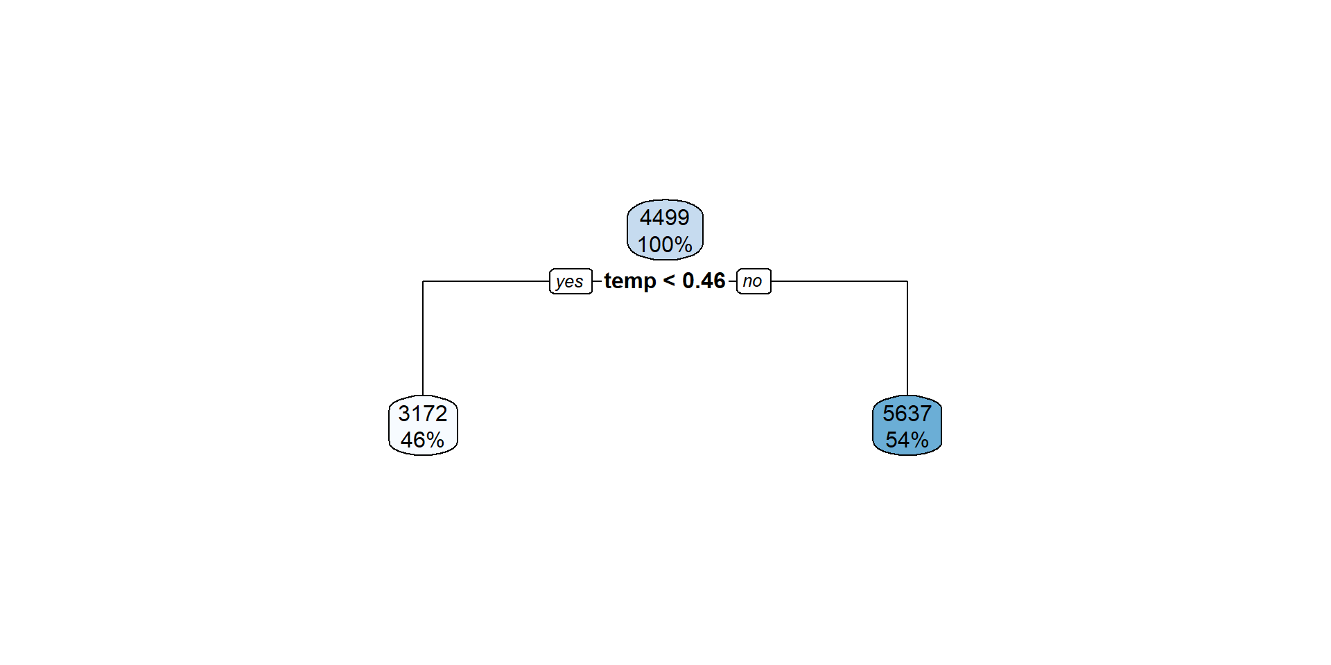
Visualize
Visualize
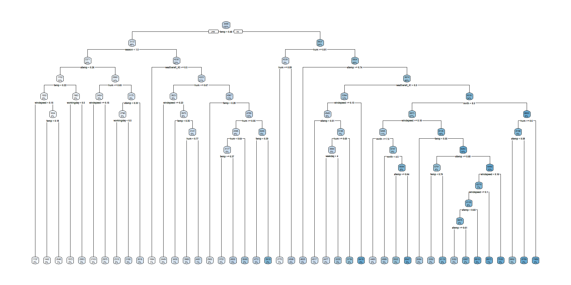
Visualize
Visualize
Defin Model Workflow with Tuning
Define Folds and Tuning Grid
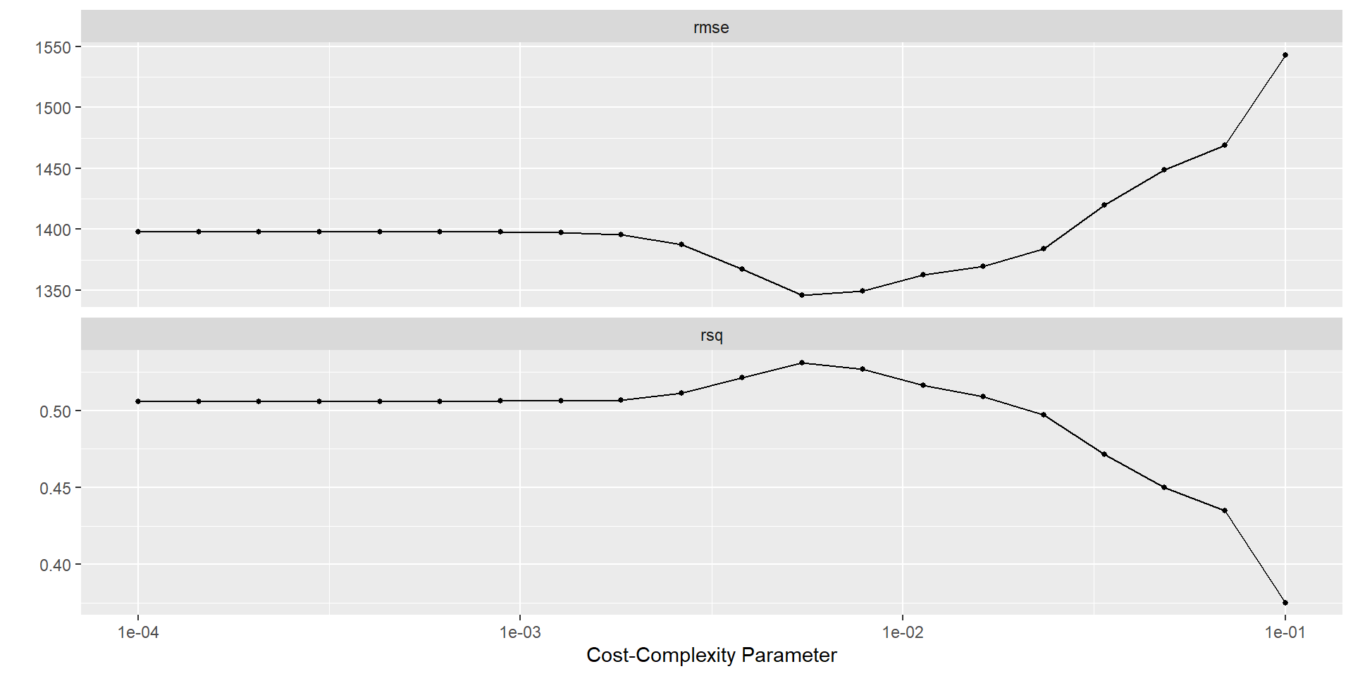
Tuning CP
Plot Results
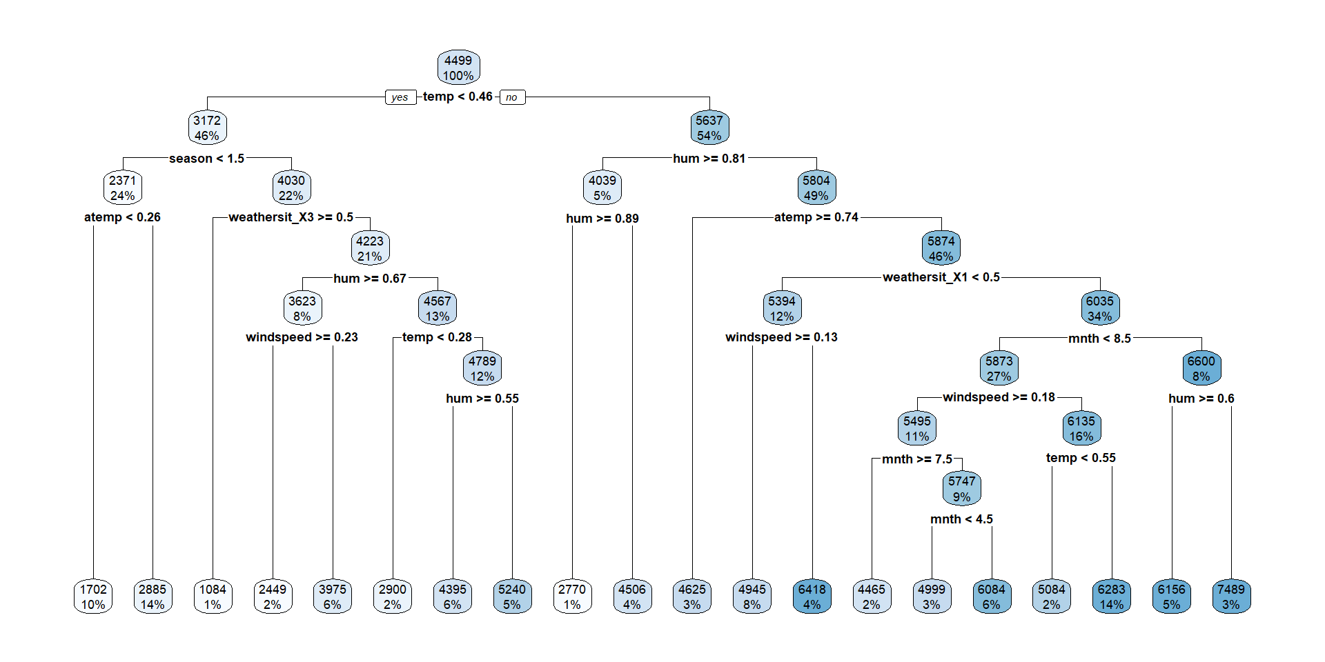
Select Best Trees
Fit Best Tree

Fit OSE Tree
Questions
- Why are both models the same but have different RMSE estimates from CV?
- What’s the difference between encoding
mnthas an ordinal variable vs. a one-hot encoding?
Decision Trees
- Advantages
- Easy to explain and interpret
- Closely mirror human decision-making
- Can be displayed graphically, and are easily interpreted by non-experts
- Does not require standardization of predictors
- Can handle missing data directly
- Can easily capture non-linear patterns
- Disadvantages
- Do not have same level of prediction accuracy
- Not very robust