MATH 427: Bagging and Boosting
Eric Friedlander
Computational Set-Up
Ensemble Methods
- Single regression or classification trees usually have poor predictive performance.
- Ensemble Methods: use a collection of models (in this case, decision trees) to improve the predictive performance
- Downside: Interpretability
- Today:
- Bagging
- Random Forests
- Boosting
Flexibility vs. Interpretability
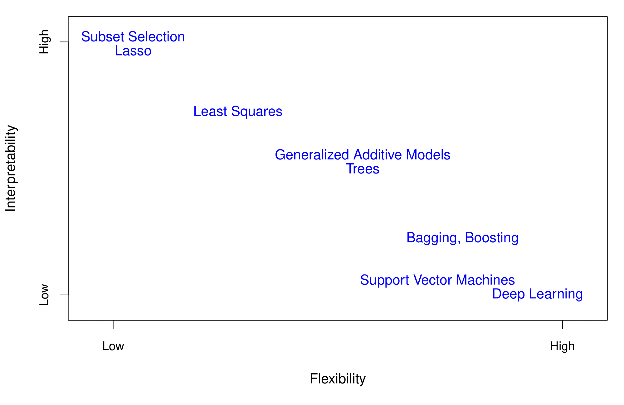
Adapted from ISLR, James et al.
Bagging
- Bootstrap aggregation or bagging is a general-purpose procedure for reducing the variance of a statistical learning method.
- Idea: Build multiple trees and average their results.
- Result: Given a set of \(n\) independent observations (random variables) \(Z_1, \ldots, Z_n\), each with variance \(\sigma^2\), the variance of the mean/average \(\bar{Z} = \displaystyle \dfrac{Z_1 + Z_2 + \cdots + Z_n}{n}\) of the observations is \(\sigma^2/n\).
- In other words, averaging a set of observations reduces variance.
- In reality, we do not have multiple training datasets.
Bootstrapping
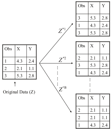
Adapted from ISLR, James et al.
Bagging
- Take repeated bootstrap samples (say \(B\)) from the original dataset.
- Build tree on each bootstrap sample and obtain predictions \(\hat{f}^{*b}(x), \ b=1, 2, \ldots, B\).
- Average all the predictions: \[\hat{f}_{\text{bag}}(x) = \frac{1}{B}\sum_{i=1}^B\hat{f}^{*b}(x)\]
- Trees not pruned: They have high variance, but low bias.
- Classification: majority vote the overall prediction is the most commonly occurring class among the \(B\) predictions
Out-of-Bag Error Estimation
- Bagging \(\Rightarrow\) fitting lots of models \(\Rightarrow\) computationally taxing
- Bagging + Cross-validation \(\Rightarrow\) EXTREMELY COMPUTATIONALLY TAXING
- On average, each bagged tree (constructed on each bootstrap sample) makes use of around two-thirds of the observations.
- Remaining third observations referred to as out-of-bag (OOB) observations
- For \(i^{th}\) observation, use the trees in which that observation was OOB. This will yield around \(B/3\) predictions for the \(i^{th}\) observation. Take their average to obtain a single prediction
- Equivalent to LOOCV if \(B\) is large
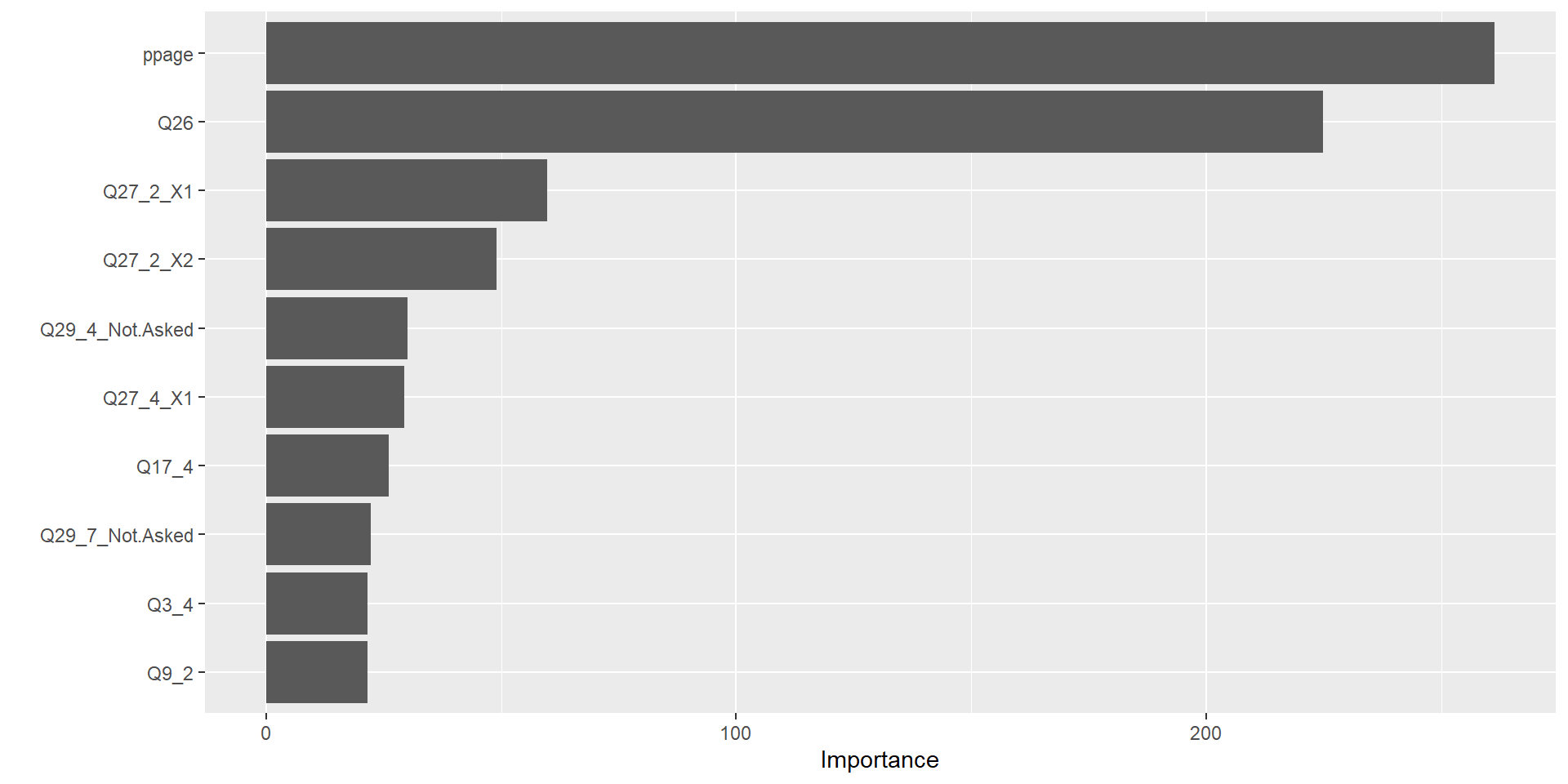
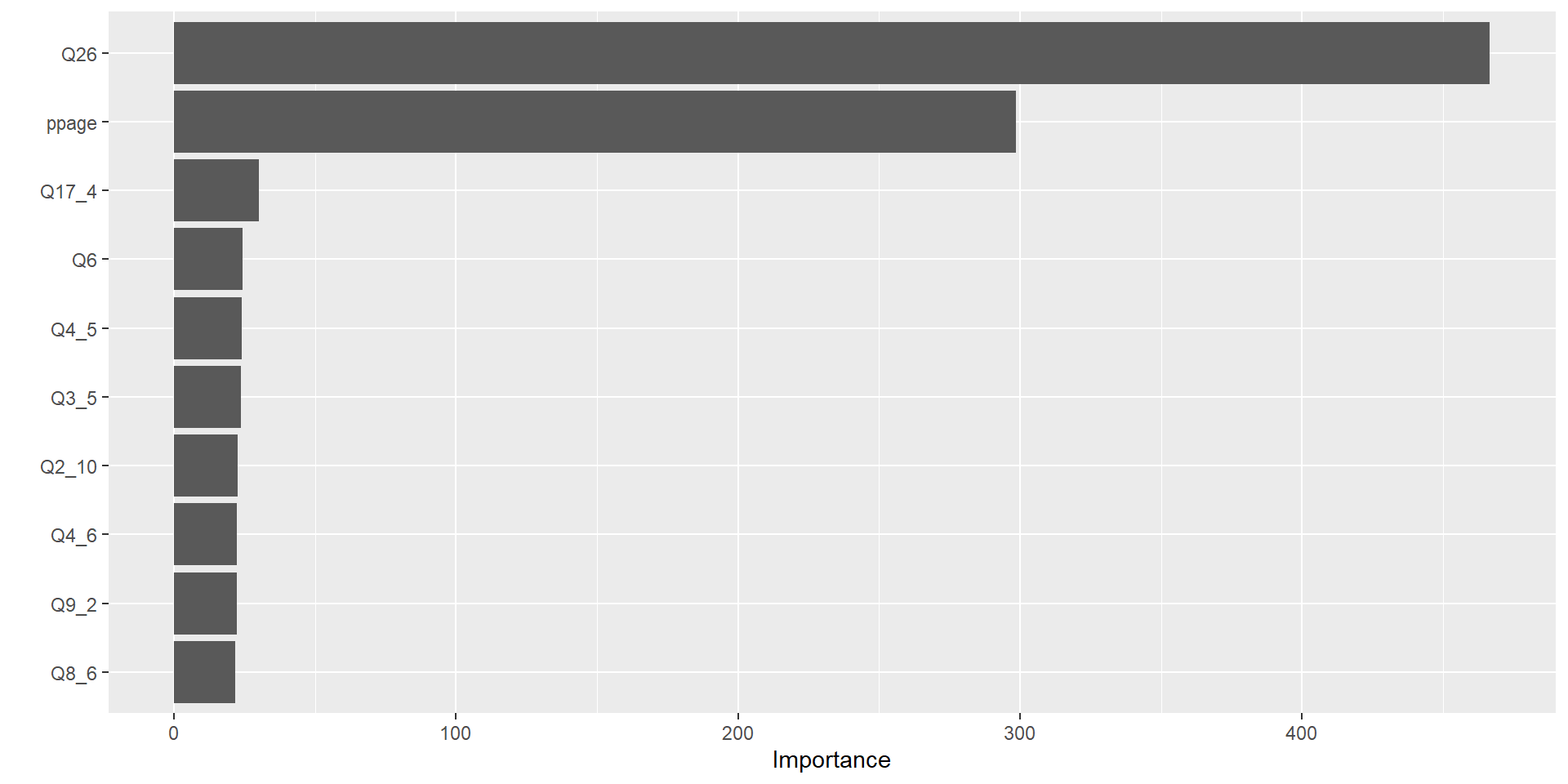
Variable Importance Measures
- Bagging improves prediction accuracy at expense of interpretability
- Can still obtain overall summary of importance of each predictor
- Reduction in the loss function (e.g., SSE) attributed to each variable at each split is tabulated
- A single variable could be used multiple times in a tree
- Total reduction in the loss function across all splits by a variable are summed up and used as the total feature importance
- A large value indicates an important predictor.
Bagging Implementation in R
Data: Voter Frequency
- Info about data
- Goal: Identify individuals who are unlikely to vote to help organization target “get out the vote” effort.
voter_data <- read_csv('https://raw.githubusercontent.com/fivethirtyeight/data/master/non-voters/nonvoters_data.csv')

voter_clean <- voter_data |>
  select(-RespId, -weight, -Q1) |>
  mutate(
    educ = factor(educ, levels = c("High school or less", "Some college", "College")),
    income_cat = factor(income_cat, levels = c("Less than $40k", "$40-75k ",
                                               "$75-125k", "$125k or more")),
    voter_category = factor(voter_category, levels = c("rarely/never", "sporadic", "always"))
  ) |>
  filter(Q22 != 5 | is.na(Q22)) |>
  mutate(Q22 = as_factor(Q22),
         Q22 = if_else(is.na(Q22), "Not Asked", Q22),
         across(Q28_1:Q28_8, ~if_else(.x == -1, 0, .x)),
         across(Q28_1:Q28_8, ~ as_factor(.x)),
         across(Q28_1:Q28_8, ~if_else(is.na(.x) , "Not Asked", .x)),
         across(Q29_1:Q29_10, ~if_else(.x == -1, 0, .x)),
         across(Q29_1:Q29_10, ~ as_factor(.x)),
         across(Q29_1:Q29_8, ~if_else(is.na(.x) , "Not Asked", .x)),
        Party_ID = as_factor(case_when(
          Q31 == 1 ~ "Strong Republican",
          Q31 == 2 ~ "Republican",
          Q32 == 1  ~ "Strong Democrat",
          Q32 == 2 ~ "Democrat",
          Q33 == 1 ~ "Lean Republican",
          Q33 == 2 ~ "Lean Democrat",
          TRUE ~ "Other"
        )),
        Party_ID = factor(Party_ID, levels =c("Strong Republican", "Republican", "Lean Republican",
                                                "Other", "Lean Democrat", "Democrat", "Strong Democrat")),
        across(!ppage, ~as_factor(if_else(.x == -1, NA, .x))))
Split Data
Define Model
trees: kind of a tuning parameter… want to select value that is large enough but doesn’t matter past that
Define Recipe
bag_recipe <- recipe(voter_category ~ . , data = voter_train) |>
  step_indicate_na(all_predictors()) |>
  step_zv(all_predictors()) |>
  step_integer(educ, income_cat, Party_ID, Q2_2:Q4_6, Q6, Q8_1:Q9_4, Q14:Q17_4,
               Q25:Q26) |>
  step_impute_median(all_numeric_predictors()) |>
  step_impute_mode(all_nominal_predictors()) |>
  step_dummy(all_nominal_predictors(), one_hot = TRUE)
Define Workflow and Fit
Evaluate performance
Variable Importance
Bagging: Disadvantages
- improves prediction performance but reduces interpretability
- trees in bagging not completely independent of each other since all the original features are considered at every split of every tree
- tree correlation: trees from different bootstrap samples typically have similar structure to each other (especially at the top of the tree)
- prevents bagging from further reducing the variance of the individual models
- Random forests extend and improve upon bagged decision trees by reducing this correlation and thereby improving the accuracy of the overall ensemble.
Bagging: Disadvantages
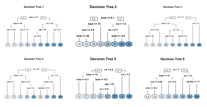
Adapted from Hands-On Machine Learning, Boehmke & Greenwell
Random Forests
Random Forests
- De-correlates bagged trees \(\Rightarrow\) reducing variance
- As in bagging, we build a number of decision trees on bootstrapped training samples.
- Algorithm: do the following to build each tree
- Generate bootstrapped sample of training data
- Randomly select \(m\) predictors
- Pick best variable/split-oint from these \(m\)
- Split node into two child nodes
- Stop when typical stopped criteria is hit (not pruning)
- Note: A fresh sample of \(m\) predictors is taken at each split
- Typically \(m = p/3\) for regression and \(m = \sqrt{p}\) for classification but this should be considered a tuning parameter
Define Model
trees: kind of a tuning parameter… want to select value that is large enough but doesn’t matter past that
Define Recipe
rf_recipe <- recipe(voter_category ~ . , data = voter_train) |>
  step_indicate_na(all_predictors()) |>
  step_zv(all_predictors()) |>
  step_integer(educ, income_cat, Party_ID, Q2_2:Q4_6, Q6, Q8_1:Q9_4, Q14:Q17_4,
               Q25:Q26) |>
  step_impute_median(all_numeric_predictors()) |>
  step_impute_mode(all_nominal_predictors()) |>
  step_dummy(all_nominal_predictors(), one_hot = TRUE)
Define Workflow and Fit
Upper Limit for mtry
Extract Number of Features
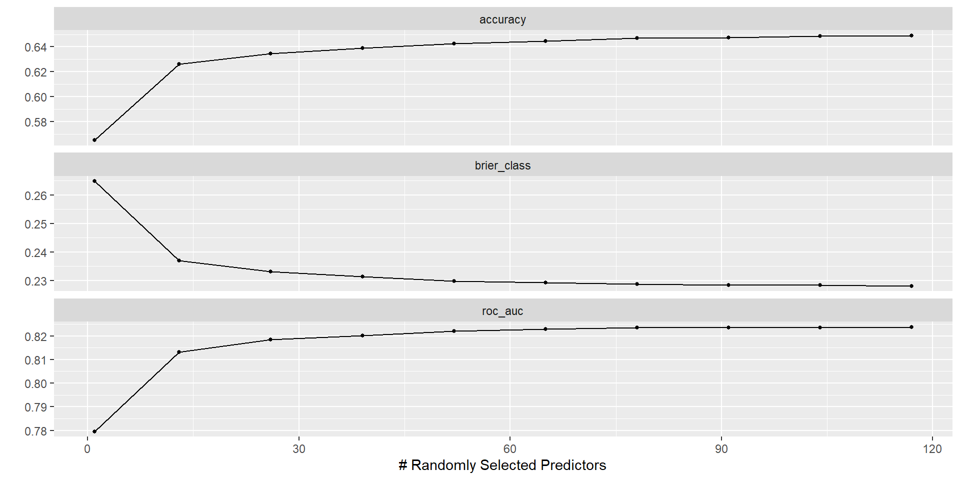
Tune mtry
Results