MATH 427: More on Classification
Eric Friedlander
Computational Set-Up
Quick Review of Classification
- We’ve covered many different classification methods:
- Logistic Regression (potentially with regularization)
- KNN
- Decision Tress
- Random Forests
- Gradient Boosted Trees
- For each of these methods, rank them as (high/medium/low) for each of the following criteria
- Computational complexity to fit
- Computational complexity to predict
- Ability to handle non-linearity
- Interpretability
- Prediction accuracy
Quick Review of Classification
| Logistic Regression | KNN | Decision Trees | Random Forests | Gradient Boosted Trees | |
|---|---|---|---|---|---|
| Comp. Fit | Low | Low | Low | Medium | High |
| Comp. Pred. | Low | Depends | Low | Medium | Medium |
| Non-linearity | Low | Medium | Medium | High | High |
| Interp. | High | Low | High | Medium/Low | Medium/Low |
| Acc. | Low | Depends | Low | Medium/High | High |
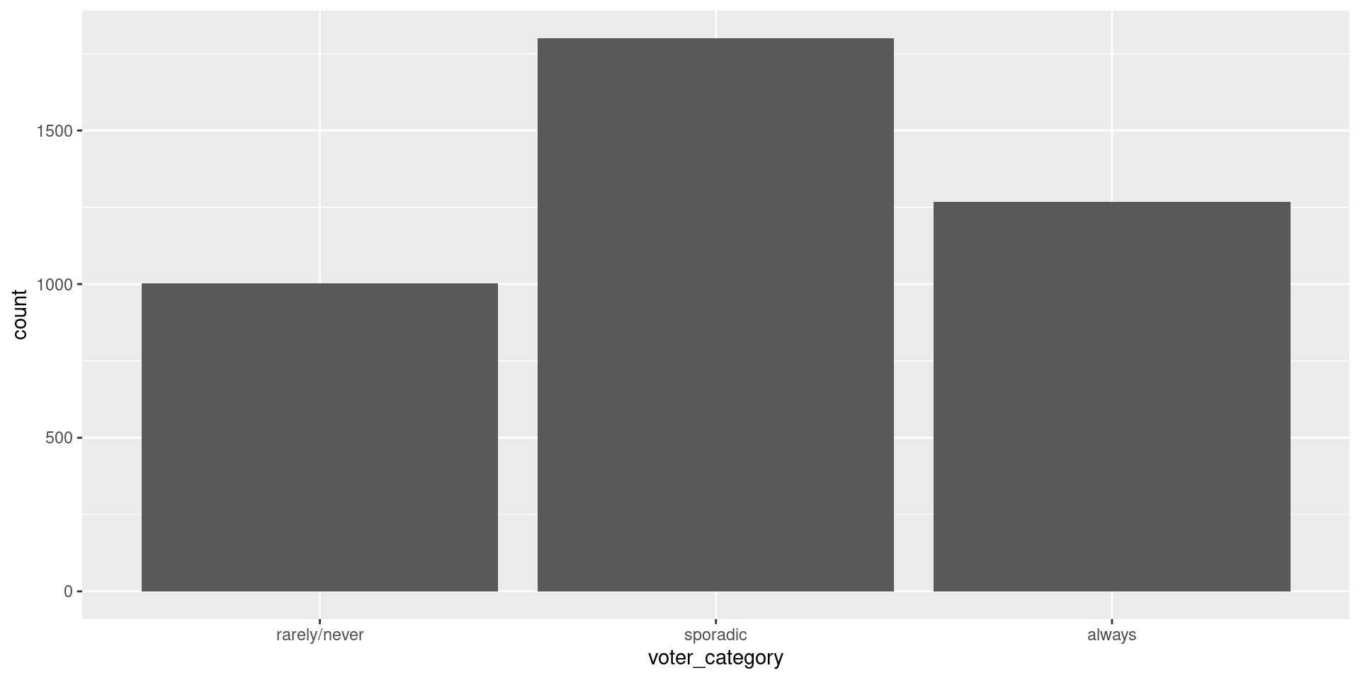
Data: Voter Frequency
- Info about data
- Goal: Identify individuals who are unlikely to vote to help organization target “get out the vote” effort.
voter_data <- read_csv('https://raw.githubusercontent.com/fivethirtyeight/data/master/non-voters/nonvoters_data.csv')

voter_clean <- voter_data |>
  select(-RespId, -weight, -Q1) |>
  mutate(
    educ = factor(educ, levels = c("High school or less", "Some college", "College")),
    income_cat = factor(income_cat, levels = c("Less than $40k", "$40-75k ",
                                               "$75-125k", "$125k or more")),
    voter_category = factor(voter_category, levels = c("rarely/never", "sporadic", "always"))
  ) |>
  filter(Q22 != 5 | is.na(Q22)) |>
  mutate(Q22 = as_factor(Q22),
         Q22 = if_else(is.na(Q22), "Not Asked", Q22),
         across(Q28_1:Q28_8, ~if_else(.x == -1, 0, .x)),
         across(Q28_1:Q28_8, ~ as_factor(.x)),
         across(Q28_1:Q28_8, ~if_else(is.na(.x) , "Not Asked", .x)),
         across(Q29_1:Q29_10, ~if_else(.x == -1, 0, .x)),
         across(Q29_1:Q29_10, ~ as_factor(.x)),
         across(Q29_1:Q29_8, ~if_else(is.na(.x) , "Not Asked", .x)),
        Party_ID = as_factor(case_when(
          Q31 == 1 ~ "Strong Republican",
          Q31 == 2 ~ "Republican",
          Q32 == 1  ~ "Strong Democrat",
          Q32 == 2 ~ "Democrat",
          Q33 == 1 ~ "Lean Republican",
          Q33 == 2 ~ "Lean Democrat",
          TRUE ~ "Other"
        )),
        Party_ID = factor(Party_ID, levels =c("Strong Republican", "Republican", "Lean Republican",
                                                "Other", "Lean Democrat", "Democrat", "Strong Democrat")),
        across(!ppage, ~as_factor(if_else(.x == -1, NA, .x))))
Split Data
Problem: More than two categories
Define Model: Multinomial Regression
Define Recipe
mr_recipe <- recipe(voter_category ~ . , data = voter_train) |>
  step_zv(all_predictors()) |>
  step_integer(educ, income_cat, Party_ID, Q2_2:Q4_6, Q6, Q8_1:Q9_4, Q14:Q17_4,
               Q25:Q26) |>
  step_impute_median(all_numeric_predictors()) |>
  step_impute_mode(all_nominal_predictors()) |>
  step_dummy(all_nominal_predictors(), one_hot = FALSE) |>
  step_normalize(all_numeric_predictors())
Define Workflow and Fit
Look at Predictions
| .pred_class | .pred_rarely/never | .pred_sporadic | .pred_always |
|---|---|---|---|
| sporadic | 0.0317402 | 0.5122327 | 0.4560271 |
| always | 0.0463060 | 0.4464935 | 0.5072005 |
| sporadic | 0.0553279 | 0.6529393 | 0.2917328 |
| always | 0.0388506 | 0.4351109 | 0.5260385 |
| always | 0.0361359 | 0.4164662 | 0.5473979 |
| always | 0.0991499 | 0.4310622 | 0.4697879 |
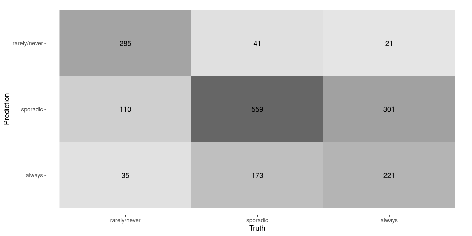
Confusion Matrix
Evaluating Multiclass Models
- No “Positive” and “Negative” anymore
- Accuracy: \[\frac{\text{Correct classifications}}{\text{total observations}} = \frac{285+559+221}{1746} \approx 0.61\]
- Most of our metrics were based on having “Positive” vs. “Negative”
- Precision/PPV
- Recall/Sensitivity
- Specificity
- NPV
- ROC/AUC
Evaluating Multiclass Models
- Solution 1: Apply binary metrics to each class in turn
- E.g. report three different Recall values
- Rarely: \(\frac{285}{285+110+35} = \approx 0.66\)
- Sporadic: \(\frac{559}{47+559+173} = \approx 0.72\)
- Always: \(\frac{221}{21+301+221} = \approx 0.41\)
- E.g. report three different Recall values
- Compute the Precision for each class:
- Reminder: Precision = TP/(TP+FP)
Solution 1 in R
- No automatic implementation in yardstick (can hack together using
group_bysometimes)
Evaluating Multiclass Models
- Solution 2: Average metrics across labels
- Macro-averaging average one-versus-all metrics
- Recall: \(\frac{0.66+0.72+0.41}{3} \approx 0.60\)
- Macro-weighted averaging same but weight by class size
- Recall: \(\frac{430\times 0.66+773\times 0.72+543\times 0.41}{1746} \approx 0.61\)
- Micro-averaging compute contribution for each class, aggregates them, then computes a single metric
- Recall: \(\frac{285+559+221}{430+779+543} \approx 0.61\)
- Macro-averaging average one-versus-all metrics
Macro-Averaging in R
Macro-Weighted Averaging in R
Micro-Averaging in R
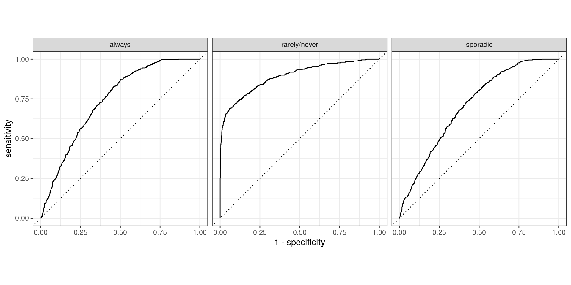
What if output is probability?
- For binary case we used ROC curve and AUC…
- Similar ideas apply here:
- One vs. all
- Macro Averaging
- NO MICRO AVERAGING!
- Hand and Till extension of AUC
Plotting one-vs.-all
Macro Averaged AUC
Macro-Weighted Averaged AUC
Hand and Till AUC
- Paper
- Basic Idea: Do pairwise comparison of classes and average
Discussion
How would heavily imbalanced classes impact each type of macro vs. micro averaging?
Dealing with Class-Imbalance
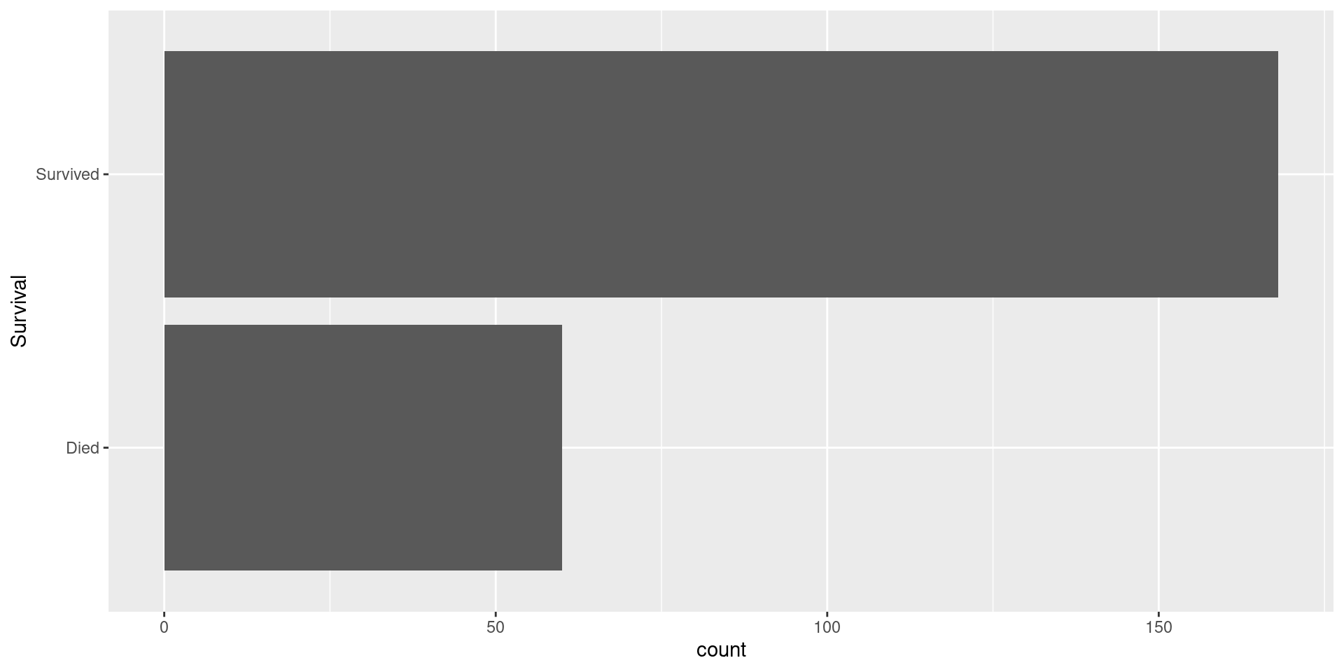
Class-Imbalance
- Class-imbalance occurs where your the classes in your response greatly differ in terms of how common they are
- Occurs frequently:
- Medicine: survival/death
- Admission: enrollment/non-enrollment
- Finance: repaid loan/defaulted
- Tech: Clicked on ad/Didn’t click
- Tech: Churn rate
- Finance: Fraud
Data: haberman
Study conducted between 1958 and 1970 at the University of Chicago’s Billings Hospital on the survival of patients who had undergone surgery for breast cancer.
Goal: predict whether a patient survived after undergoing surgery for breast cancer.
haberman <- read_csv("../data/haberman.data",
                     col_names = c("Age", "OpYear", "AxNodes", "Survival"))
glimpse(haberman)
Rows: 306
Columns: 4
$ Age <dbl> 30, 30, 30, 31, 31, 33, 33, 34, 34, 34, 34, 34, 34, 34, 35, 3…
$ OpYear <dbl> 64, 62, 65, 59, 65, 58, 60, 59, 66, 58, 60, 61, 67, 60, 64, 6…
$ AxNodes <dbl> 1, 3, 0, 2, 4, 10, 0, 0, 9, 30, 1, 10, 7, 0, 13, 0, 1, 0, 0, …
$ Survival <dbl> 1, 1, 1, 1, 1, 1, 1, 2, 2, 1, 1, 1, 1, 1, 1, 1, 1, 1, 1, 1, 1…Quick Clean
Study conducted between 1958 and 1970 at the University of Chicago’s Billings Hospital on the survival of patients who had undergone surgery for breast cancer.
Goal: predict whether a patient died after undergoing surgery for breast cancer.
haberman <- haberman |>
  mutate(Survival = factor(if_else(Survival == 1, "Survived", "Died"),
                           levels = c("Died", "Survived")))
glimpse(haberman)
Rows: 306
Columns: 4
$ Age <dbl> 30, 30, 30, 31, 31, 33, 33, 34, 34, 34, 34, 34, 34, 34, 35, 3…
$ OpYear <dbl> 64, 62, 65, 59, 65, 58, 60, 59, 66, 58, 60, 61, 67, 60, 64, 6…
$ AxNodes <dbl> 1, 3, 0, 2, 4, 10, 0, 0, 9, 30, 1, 10, 7, 0, 13, 0, 1, 0, 0, …
$ Survival <fct> Survived, Survived, Survived, Survived, Survived, Survived, S…Split Data
Visualizing Response
Fitting Model
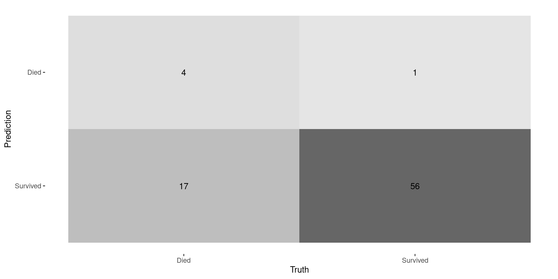
Confusion Matrix
Performance Metrics
hab_metrics <- metric_set(accuracy, precision, recall)

lr_fit |> augment(new_data = hab_test) |>
roc_auc(truth = Survival, .pred_Died) |> kable()| .metric | .estimator | .estimate |
|---|---|---|
| roc_auc | binary | 0.7284879 |
lr_fit |> augment(new_data = hab_test) |>
hab_metrics(truth = Survival, estimate = .pred_class) |> kable()| .metric | .estimator | .estimate |
|---|---|---|
| accuracy | binary | 0.7692308 |
| precision | binary | 0.8000000 |
| recall | binary | 0.1904762 |
Recall is BAD!
- Since there are so few deaths, model always predicts a low probability of death
- Idea: just because you you have a HIGHER probability of death doesn’t mean have a HIGH probability of death
What do we do?
- Depends on what your goal is…
- Ask yourself: What is most important to my problem?
- Accurate probabilities?
- Effective Separation?
- Effective identification of positives?
- Low false-positive rate?
- Discussion: Let’s think of scenarios where each one of these is the most important.