MATH 427: Class Imbalance

Eric Friedlander

Computational Set-Up

library(tidyverse)
library(tidymodels)
library(knitr)
library(kableExtra)

tidymodels_prefer()

set.seed(427)

Exploring with App

• App
  • Break into groups
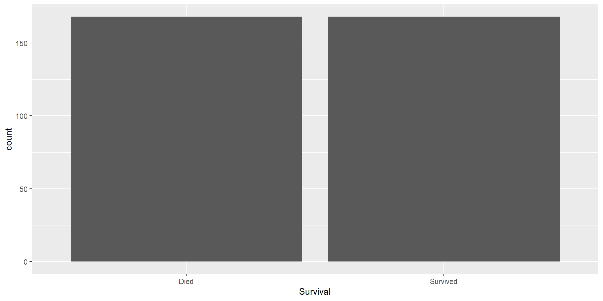
  • Investigate how your performance metrics change between balanced data and unbalanced data
  • Additional Considerations:
    • Impact of boundaries/models?
    • Impact of sample size?
    • Impact of noise level?
  • Please write down observations so we can discuss

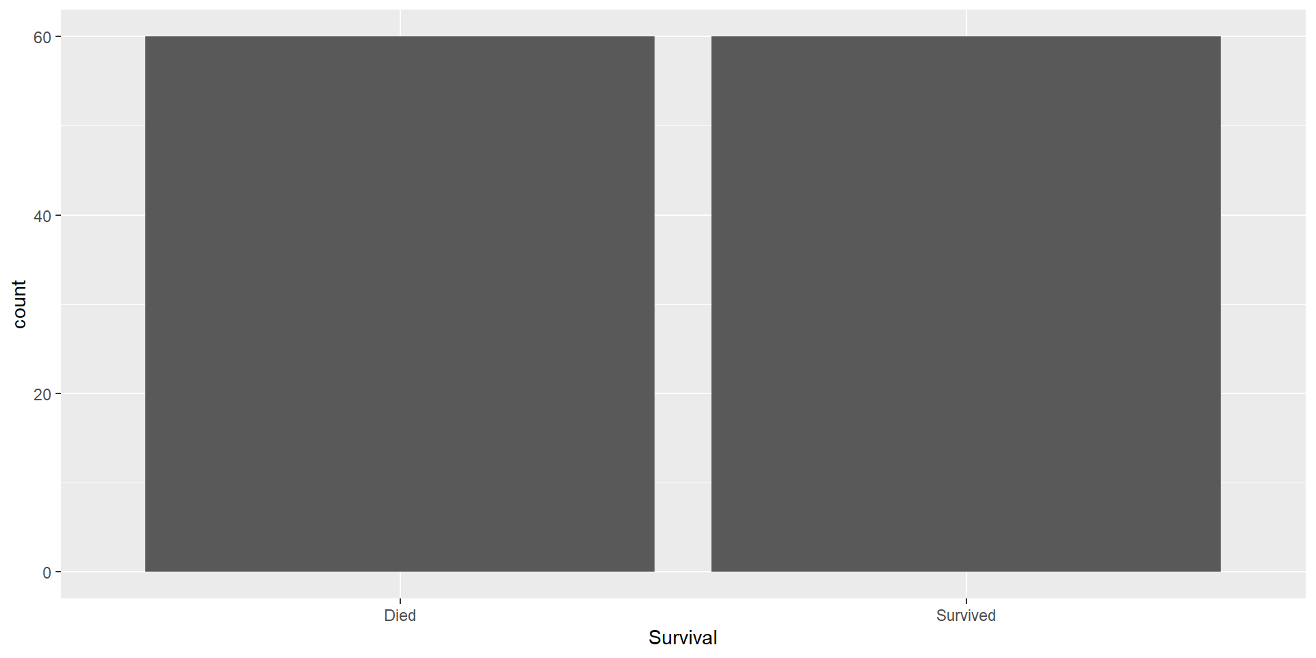
Dealing with Class-Imbalance

Class-Imbalance

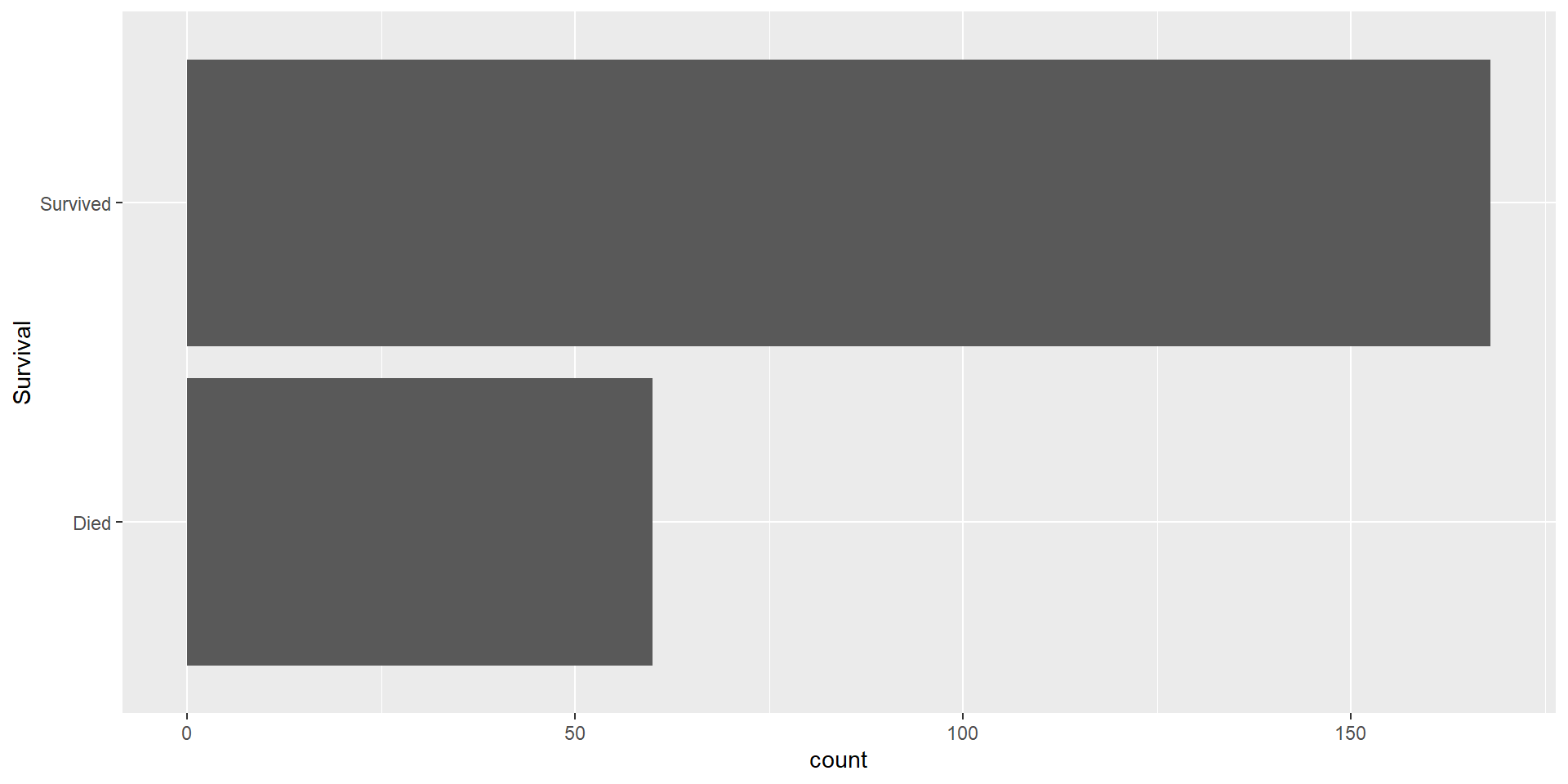
• Class-imbalance occurs where your the classes in your response greatly differ in terms of how common they are
• Occurs frequently:
  • Medicine: survival/death
  • Admissions: enrollment/non-enrollment
  • Finance: repaid loan/defaulted
  • Tech: Clicked on ad/Didn’t click
  • Tech: Churn rate
  • Finance: Fraud

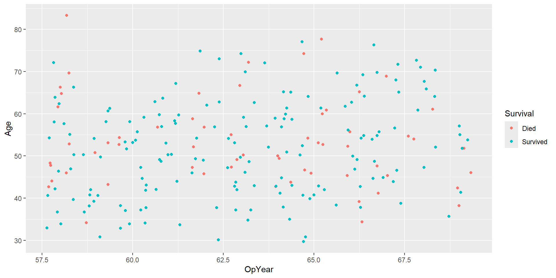
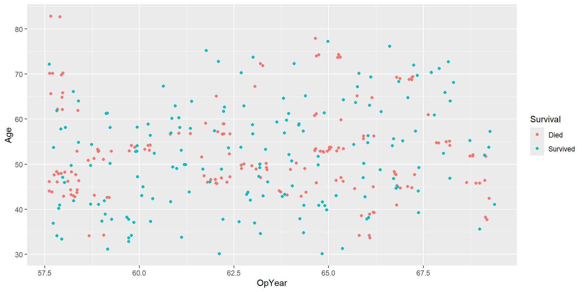
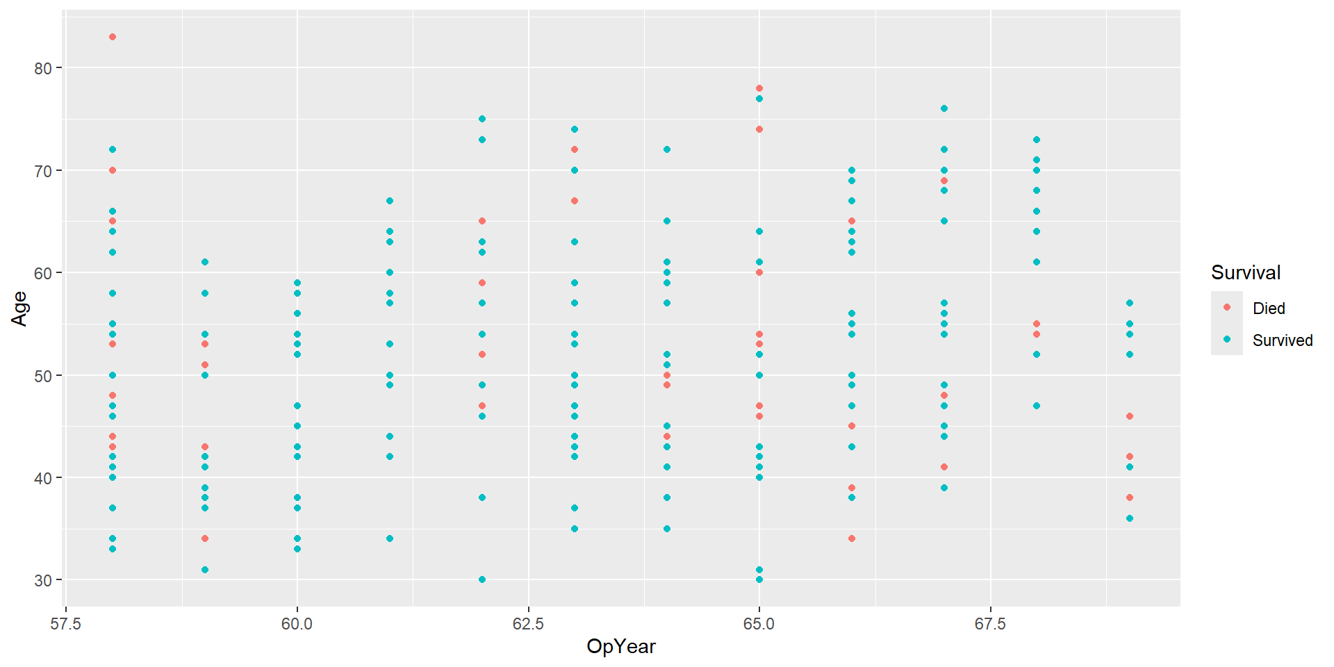
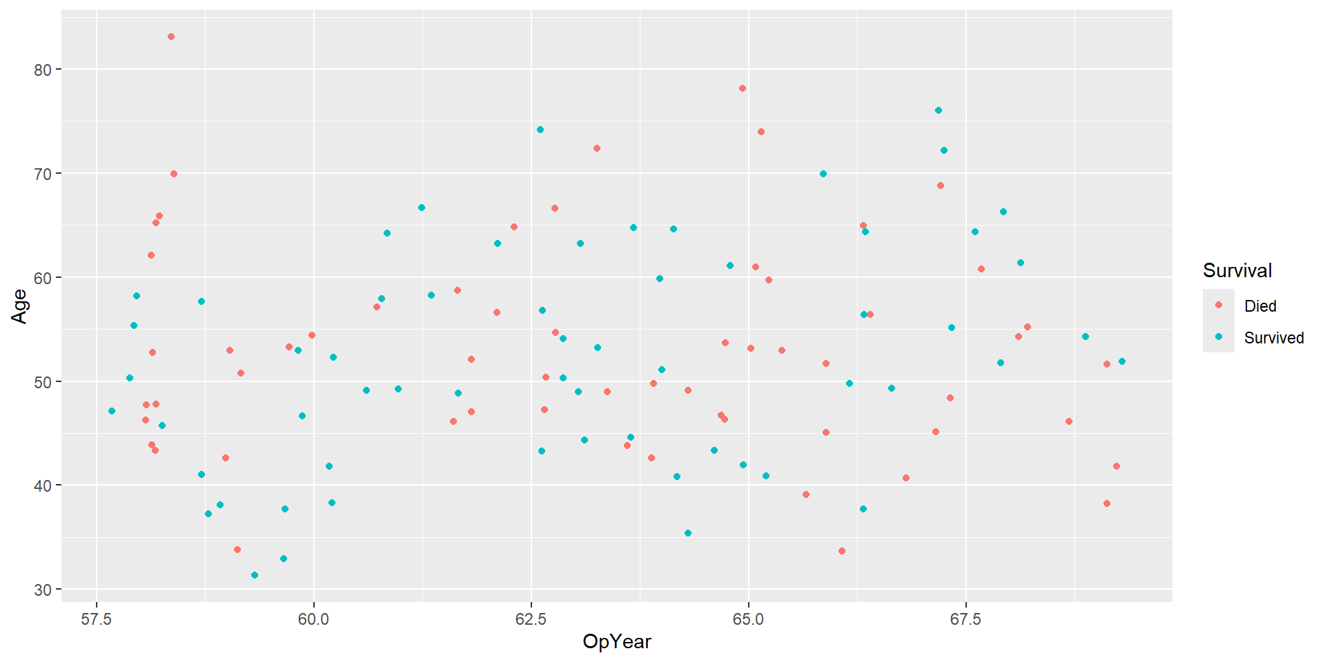
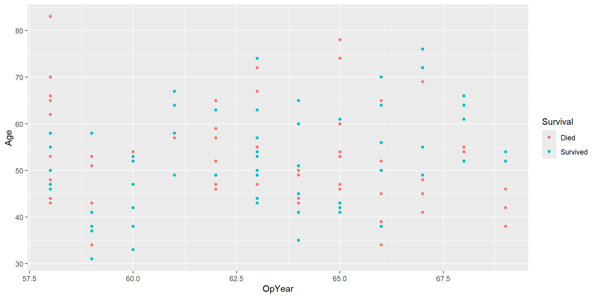
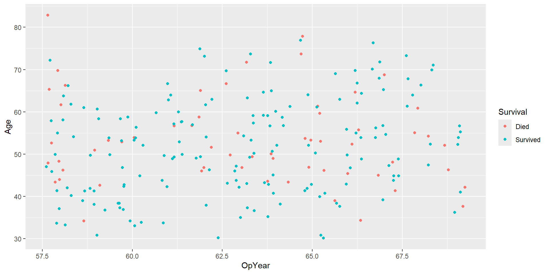
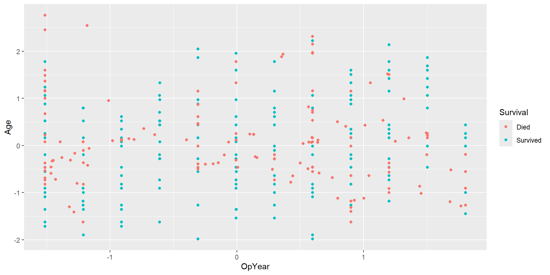
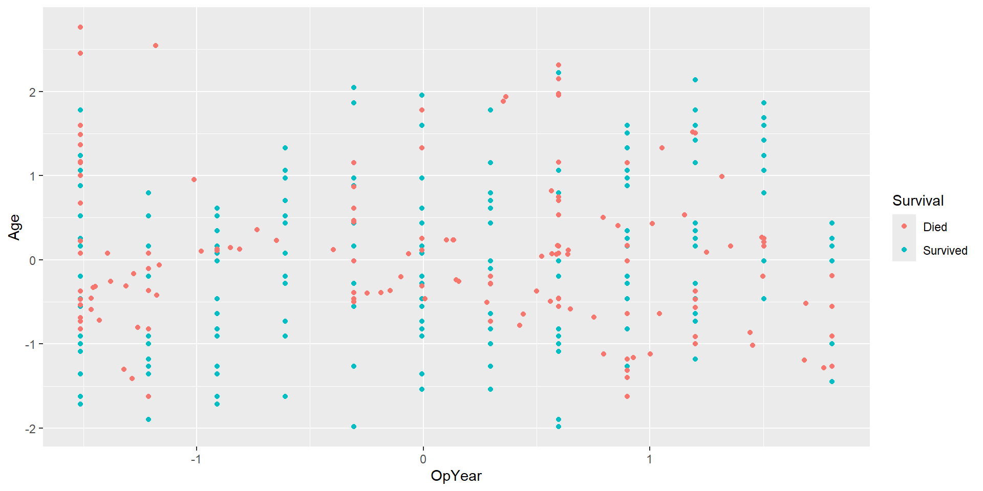
Data: haberman

Study conducted between 1958 and 1970 at the University of Chicago’s Billings Hospital on the survival of patients who had undergone surgery for breast cancer.

Goal: predict whether a patient survived after undergoing surgery for breast cancer.

haberman <- read_csv("../data/haberman.data",
                     col_names = c("Age", "OpYear", "AxNodes", "Survival"))
haberman |> head() |> kable()

Age	OpYear	AxNodes	Survival
30	64	1	1
30	62	3	1
30	65	0	1
31	59	2	1
31	65	4	1
33	58	10	1

Quick Clean

haberman <- haberman |> 
  mutate(Survival = factor(if_else(Survival == 1, "Survived", "Died"),
                           levels = c("Died", "Survived")))
haberman |> head() |> kable()

Age	OpYear	AxNodes	Survival
30	64	1	Survived
30	62	3	Survived
30	65	0	Survived
31	59	2	Survived
31	65	4	Survived
33	58	10	Survived

Split Data

set.seed(427)
hab_splits <- initial_split(haberman, prop = 0.75, strata = Survival)
hab_train <- training(hab_splits)
hab_test <- testing(hab_splits)

Visualizing Response

hab_train |> 
  ggplot(aes(y = Survival)) +
  geom_bar()

Fitting Model

lr_model <- logistic_reg() |> 
  set_engine("glm")

lr_fit <- lr_model |> 
  fit(Survival ~ . , data = hab_train)

Confusion Matrix

lr_fit |> augment(new_data = hab_test) |> 
  conf_mat(truth = Survival, estimate = .pred_class) |> autoplot("heatmap")

Performance Metrics

hab_metrics <- metric_set(accuracy, precision, recall)

lr_fit |> augment(new_data = hab_test) |> 
  roc_auc(truth = Survival, .pred_Died) |> kable()

.metric	.estimator	.estimate
roc_auc	binary	0.7284879

lr_fit |> augment(new_data = hab_test) |> 
  hab_metrics(truth = Survival, estimate = .pred_class) |> kable()

.metric	.estimator	.estimate
accuracy	binary	0.7692308
precision	binary	0.8000000
recall	binary	0.1904762

Recall is BAD!

• Since there are so few deaths, model always predicts a low probability of death
• Idea: just because you you have a HIGHER probability of death doesn’t mean have a HIGH probability of death

What do we do?

• Depends on what your goal is…
• Ask yourself: What is most important to my problem?
  • Accurate probabilities?
  • Overall accuracy?
  • Effective identification of a specific class (e.g. positives)?
  • Low false-positive rate?
• Discussion: Let’s think of scenarios where each one of these is the most important.

Solutions to Class Imbalance

• Adjust probability threshold (we’ve already done this)
  • If you wanted to increase your recall would you increase or decrease your threshold?
• Sampling-based solutions (done during pre-processing)
  • Over-sample minority class
  • Under-sample majority class
  • Combination of both (e.g. SMOTE)
• Weight class/objective function

Over-sampling minority class

• Upsample: think bootstrapping for final sample is larger than original
• Idea: upsample minority class until it is same size(ish) as majority class

Visualizing Data

hab_train |> ggplot(aes(x = OpYear, y = Age, color = Survival)) +
  geom_jitter()

Upsample Recipe

library(themis)
upsample_recipe <- recipe(Survival ~ ., data = hab_train) |> 
  step_upsample(Survival, over_ratio = 1)

hab_upsample <- upsample_recipe |> prep(hab_train) |> bake(new_data = NULL)

Upsampled Data

hab_upsample |>  ggplot(aes(x = Survival)) +
  geom_bar()

Visualizing Upsampled Data

hab_upsample |>  ggplot(aes(x = OpYear, y = Age, color = Survival)) +
  geom_jitter()

Visualizing Upsampled Data: No Jitter

hab_upsample |>  ggplot(aes(x = OpYear, y = Age, color = Survival)) +
  geom_point()

Performance consideration

• Pro:
  • Preserves all information in the data set
• Con:
  • Models will probably over-align to the noise in the minority class

Under-sampling majority class

• Downsample: collect a random sample smaller than the original sample
• Idea: down sample majority class until it is same size(ish) as minority class

Visualizing Data

hab_train |> ggplot(aes(x = OpYear, y = Age, color = Survival)) +
  geom_jitter()

Downsample Recipe

downsample_recipe <- recipe(Survival ~ ., data = hab_train) |> 
  step_downsample(Survival, under_ratio = 1)

hab_downsample <- downsample_recipe |> prep(hab_train) |> bake(new_data = NULL)

Downsample Data

hab_downsample |>  ggplot(aes(x = Survival)) +
  geom_bar()

Visualizing Downsampled Data

hab_downsample |>  ggplot(aes(x = OpYear, y = Age, color = Survival)) +
  geom_jitter()

Visualizing Downsampled Data: No Jitter

hab_downsample |>  ggplot(aes(x = OpYear, y = Age, color = Survival)) +
  geom_point()

Performance considerations

• Pro:
  • Model doesn’t over-align to noise in minority class
• Con:
  • Lose information from majority class

SMOTE

• Basic idea:
  • Both upsample minority and downsample majority (Tidymodel implementation only upsamples)
• Better Upsampling: Instead of just randomly replicating minority observations
  • Find (minority) nearest neighbors of each minority observation
  • Interpolate line between them
  • Upsample by randomly generating points in interpolated lines

Visualizing Data

hab_train |> ggplot(aes(x = OpYear, y = Age, color = Survival)) +
  geom_jitter()

SMOTE Recipe

smote_recipe <- recipe(Survival ~ ., data = hab_train) |> 
  step_normalize(all_numeric_predictors()) |> 
  step_smote(Survival, over_ratio = 1, neighbors = 5)

hab_smote <- smote_recipe |> prep(hab_train) |> bake(new_data = NULL)

SMOTE Data

hab_smote |>  ggplot(aes(x = Survival)) +
  geom_bar()

Visualizing SMOTE Data

hab_smote |>  ggplot(aes(x = OpYear, y = Age, color = Survival)) +
  geom_jitter()

Visualizing SMOTE Data: No Jitter

hab_smote |>  ggplot(aes(x = OpYear, y = Age, color = Survival)) +
  geom_point()

Performance considerations

• Pro:
  • Model doesn’t over-align (as much) to noise in minority class
  • Don’t lose (as much) information from majority class
• Con:
  • Creating new information out of nowhere

Fitting models

oversamp_fit <- workflow() |> add_recipe(upsample_recipe) |> 
  add_model(lr_model) |> fit(hab_train)
downsamp_fit <- workflow() |> add_recipe(downsample_recipe) |> 
  add_model(lr_model)  |> fit(hab_train)
smote_fit <- workflow() |> add_recipe(smote_recipe) |> 
  add_model(lr_model)  |> fit(hab_train)

Evaluate Performance

oversamp_fit |> augment(new_data = hab_test) |> 
  roc_auc(truth = Survival, .pred_Died) |> kable()

.metric	.estimator	.estimate
roc_auc	binary	0.7343358

downsamp_fit |> augment(new_data = hab_test) |> 
  roc_auc(truth = Survival, .pred_Died) |> kable()

.metric	.estimator	.estimate
roc_auc	binary	0.7243108

smote_fit |> augment(new_data = hab_test) |> 
  roc_auc(truth = Survival, .pred_Died) |> kable()

.metric	.estimator	.estimate
roc_auc	binary	0.7251462

Evaluate Performance

oversamp_fit |> augment(new_data = hab_test) |> 
  hab_metrics(truth = Survival, estimate = .pred_class) |> kable()

.metric	.estimator	.estimate
accuracy	binary	0.7692308
precision	binary	0.5714286
recall	binary	0.5714286

downsamp_fit |> augment(new_data = hab_test) |> 
  hab_metrics(truth = Survival, estimate = .pred_class) |> kable()

.metric	.estimator	.estimate
accuracy	binary	0.7435897
precision	binary	0.5217391
recall	binary	0.5714286

smote_fit |> augment(new_data = hab_test) |> 
  hab_metrics(truth = Survival, estimate = .pred_class) |> kable()

.metric	.estimator	.estimate
accuracy	binary	0.7435897
precision	binary	0.5217391
recall	binary	0.5714286

Weighting Observations/Objective Function

Creating Importance Weights

library(hardhat)
hab_train <- hab_train |> 
  mutate(weights = ifelse(Survival == "Died", 4, 1),
         weights = importance_weights(weights))

hab_train |> head() |> kable()

Age	OpYear	AxNodes	Survival	weights
34	59	0	Died	4
34	66	9	Died	4
38	69	21	Died	4
39	66	0	Died	4
41	67	0	Died	4
42	69	1	Died	4

Weighted Workflow

weighted_wf <- workflow() |> 
  add_model(lr_model) |> 
  add_recipe(recipe(Survival ~ ., data = hab_train)) |> 
  add_case_weights(weights)

weighted_fit <- weighted_wf |> 
  fit(hab_train)

Model Performance

weighted_fit |> augment(new_data = hab_test) |> 
  conf_mat(truth = Survival, estimate = .pred_class) |> autoplot("heatmap")

Model Performance

weighted_fit |> augment(new_data = hab_test) |> 
  hab_metrics(truth = Survival, estimate = .pred_class) |> kable()

.metric	.estimator	.estimate
accuracy	binary	0.5256410
precision	binary	0.3461538
recall	binary	0.8571429

weighted_fit |> augment(new_data = hab_test) |> 
  roc_auc(truth = Survival, .pred_Died) |> kable()

.metric	.estimator	.estimate
roc_auc	binary	0.7142857

Final Note / Alternative Metrics

Model vs Decisions

• Helpful framework for thinking about this:
  • Divide model predictions from decisions
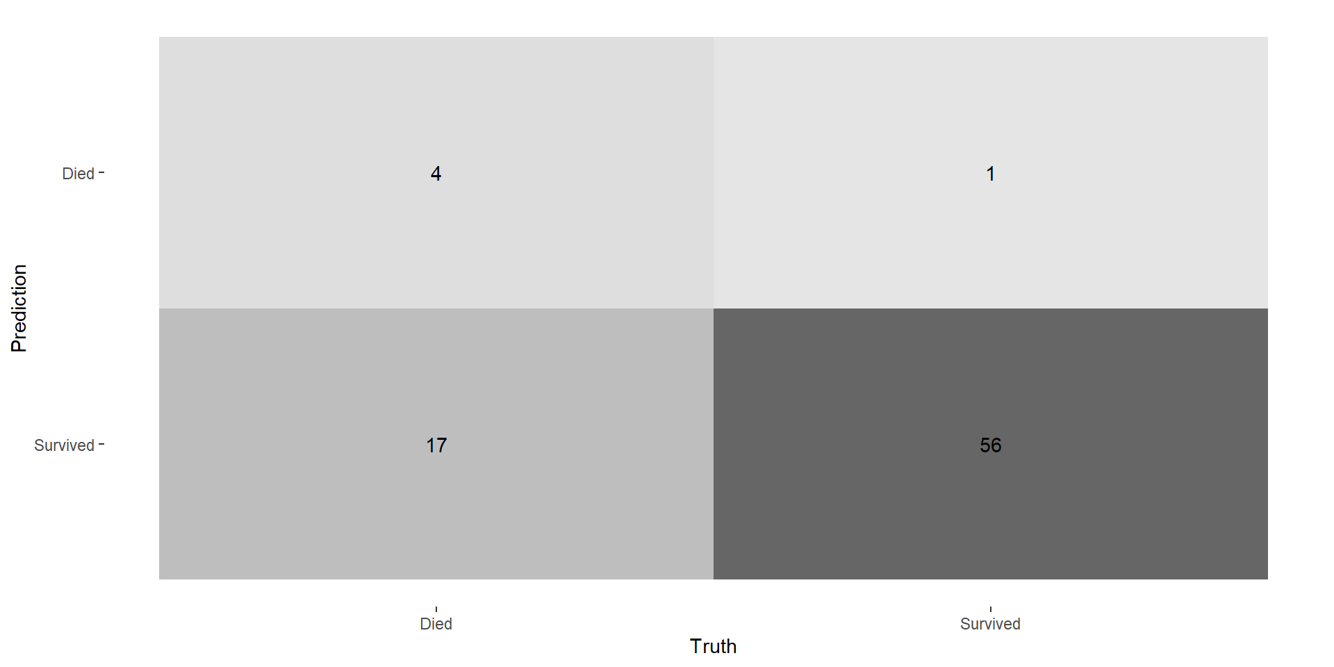
  • Usually, model predicts a probability, then you make a classification based on that probability
  • Choosing the best model probably means (1) calibrating your probabilities correctly, then (2) making classifications/decisions to optimze your use-case

Scoring Rules

• Scoring rule: metric that evaluates probabilities
• Notation:
  • \(\hat{p}_{ik}\): predicted probability observation \(i\) is in class \(k\)
  • \(y_{ik}\): 1 if observation \(i\) is in class \(k\), 0 otherwise
  • \(K\): number of classes
  • \(N\): number of observations
• Brier Score: think MSE for probabilities
  • Binary: \(\frac{1}{N} \sum_{i=1}^{N} (\hat{p}_i - y_i)^2\)
  • Multiclass: \(\frac{1}{N} \sum_{i=1}^{N} \sum_{k=1}^{K} (\hat{p}_{ik} - y_{ik})^2\)
• Logorithmic Score:
  • Binary: \(-\frac{1}{N} \sum_{i=1}^{N} \left[ y_i \log(\hat{p}_i) + (1 - y_i) \log(1 - \hat{p}_i) \right]\)
  • Multi-class: \(-\frac{1}{N} \sum_{i=1}^{N} \sum_{k=1}^{K} y_{ik} \log(\hat{p}_{ik})\)

Scoring our models

hab_scores <- metric_set(brier_class, mn_log_loss, roc_auc)
all_scores <- lr_fit |> augment(new_data = hab_test) |> hab_scores(truth = Survival, .pred_Died) |> mutate(model = "Logistic") |> 
  bind_rows(oversamp_fit |> augment(new_data = hab_test) |> hab_scores(truth = Survival, .pred_Died) |> mutate(model = "Oversample")) |> 
  bind_rows(downsamp_fit |> augment(new_data = hab_test) |> hab_scores(truth = Survival, .pred_Died) |> mutate(model = "Undersample")) |> 
  bind_rows(smote_fit |> augment(new_data = hab_test) |> hab_scores(truth = Survival, .pred_Died) |> mutate(model = "SMOTE")) |> 
  bind_rows(weighted_fit |> augment(new_data = hab_test) |> hab_scores(truth = Survival, .pred_Died) |> mutate(model = "Weighted"))

Scores

all_scores |>
  select(-.estimator) |> 
  pivot_wider(names_from = .metric, values_from = .estimate) |> 
  kable()

model	brier_class	mn_log_loss	roc_auc
Logistic	0.1678374	0.5161121	0.7284879
Oversample	0.2115716	0.6217420	0.7343358
Undersample	0.2130135	0.6298389	0.7243108
SMOTE	0.2169736	0.6304324	0.7251462
Weighted	0.2599917	0.7217460	0.7142857

Conclusion

• Many different approaches and strategies depending on data
• First strategy: tresholding
• Many times method depends on model algorithm
• Make sure to ask “Is imbalance really a problem here?”