MATH 427: Principal Component Analysis (PCA)
Eric Friedlander
Remainder of Semester
- Project (Due Friday)
- Hack-a-thon (Next week + Final Exam Time)
- Job Application 2 (Due Next Friday)
- Two Technical Interviews…
- TOO MUCH!!!
Lesson’s Learned by Dr. F
- Learning objectives coming in:
- Machine Learning Theory
- Professional Development
- Communication!!!
- Do less to do more… don’t need multiple assignments for each of these
- Prioritize an assessment before Spring Break
- Build in better time-management and revision checkpoints
Next Time
- First half of semester focused on ML pipeline and professional development
- Assess with written exam before Spring Break
- Resume and Cover Letter due before Spring Break
- Second half of semester focus on different models and communication
- Behavioral Interview shortly after Spring Break
- Sample Analysis due last week of class with draft due earlier and opportunities to revise
- Technical interview during final’s week
- Not sure about Hack-a-thon and Project
- Want to do both but feels like that is too much
Proposal For Rest of Semester
- If you like original syllabus, feel free to stick with it (no penalty)
- Project - still due Friday
- One-pager
- Presentation
Job Application 2: Hack-a-thon report- Hack-a-thon - still next week
Presentation- Predictions and report due during final exam period
- Hack-a-thon report counts as second Job Application
- Technical interviews:
- 45 minute technical interview during final exam week will replace your first technical interview grade if you do better… even if you don’t do the first interview
- Think of first interview as “practice”
New Grade Structure (Proposal)
| Category | Percentage |
|---|---|
| Homework | 10% |
| Job Application 1 | 15% |
| Job Interview 1 | 15% |
| Job Interview 2 | 20% |
| Hack-a-thon + Report | 25% |
| Project | 15% |
Computational Set-Up
Data: mnist
- MNIST Database: Modified National Institute of Standards and Technology Database
- Large database of handwritten digits
- 60,000 training images
- 10,000 test images
- Each image:
- 28x28 black and white pixels
- \(28\times 28\times 1 = 784\)
Loading data
library(dslabs)
mnist <- read_mnist()
mnist_train <- mnist$train$images
mnist_train |> head() |> kable()| 0 | 0 | 0 | 0 | 0 | 0 | 0 | 0 | 0 | 0 | 0 | 0 | 0 | 0 | 0 | 0 | 0 | 0 | 0 | 0 | 0 | 0 | 0 | 0 | 0 | 0 | 0 | 0 | 0 | 0 | 0 | 0 | 0 | 0 | 0 | 0 | 0 | 0 | 0 | 0 | 0 | 0 | 0 | 0 | 0 | 0 | 0 | 0 | 0 | 0 | 0 | 0 | 0 | 0 | 0 | 0 | 0 | 0 | 0 | 0 | 0 | 0 | 0 | 0 | 0 | 0 | 0 | 0 | 0 | 0 | 0 | 0 | 0 | 0 | 0 | 0 | 0 | 0 | 0 | 0 | 0 | 0 | 0 | 0 | 0 | 0 | 0 | 0 | 0 | 0 | 0 | 0 | 0 | 0 | 0 | 0 | 0 | 0 | 0 | 0 | 0 | 0 | 0 | 0 | 0 | 0 | 0 | 0 | 0 | 0 | 0 | 0 | 0 | 0 | 0 | 0 | 0 | 0 | 0 | 0 | 0 | 0 | 0 | 0 | 0 | 0 | 0 | 0 | 0 | 0 | 0 | 0 | 0 | 0 | 0 | 0 | 0 | 0 | 0 | 0 | 0 | 0 | 0 | 0 | 0 | 0 | 0 | 0 | 0 | 0 | 0 | 0 | 3 | 18 | 18 | 18 | 126 | 136 | 175 | 26 | 166 | 255 | 247 | 127 | 0 | 0 | 0 | 0 | 0 | 0 | 0 | 0 | 0 | 0 | 0 | 0 | 30 | 36 | 94 | 154 | 170 | 253 | 253 | 253 | 253 | 253 | 225 | 172 | 253 | 242 | 195 | 64 | 0 | 0 | 0 | 0 | 0 | 0 | 0 | 0 | 0 | 0 | 0 | 49 | 238 | 253 | 253 | 253 | 253 | 253 | 253 | 253 | 253 | 251 | 93 | 82 | 82 | 56 | 39 | 0 | 0 | 0 | 0 | 0 | 0 | 0 | 0 | 0 | 0 | 0 | 0 | 18 | 219 | 253 | 253 | 253 | 253 | 253 | 198 | 182 | 247 | 241 | 0 | 0 | 0 | 0 | 0 | 0 | 0 | 0 | 0 | 0 | 0 | 0 | 0 | 0 | 0 | 0 | 0 | 0 | 80 | 156 | 107 | 253 | 253 | 205 | 11 | 0 | 43 | 154 | 0 | 0 | 0 | 0 | 0 | 0 | 0 | 0 | 0 | 0 | 0 | 0 | 0 | 0 | 0 | 0 | 0 | 0 | 0 | 14 | 1 | 154 | 253 | 90 | 0 | 0 | 0 | 0 | 0 | 0 | 0 | 0 | 0 | 0 | 0 | 0 | 0 | 0 | 0 | 0 | 0 | 0 | 0 | 0 | 0 | 0 | 0 | 0 | 0 | 139 | 253 | 190 | 2 | 0 | 0 | 0 | 0 | 0 | 0 | 0 | 0 | 0 | 0 | 0 | 0 | 0 | 0 | 0 | 0 | 0 | 0 | 0 | 0 | 0 | 0 | 0 | 0 | 11 | 190 | 253 | 70 | 0 | 0 | 0 | 0 | 0 | 0 | 0 | 0 | 0 | 0 | 0 | 0 | 0 | 0 | 0 | 0 | 0 | 0 | 0 | 0 | 0 | 0 | 0 | 0 | 0 | 35 | 241 | 225 | 160 | 108 | 1 | 0 | 0 | 0 | 0 | 0 | 0 | 0 | 0 | 0 | 0 | 0 | 0 | 0 | 0 | 0 | 0 | 0 | 0 | 0 | 0 | 0 | 0 | 0 | 81 | 240 | 253 | 253 | 119 | 25 | 0 | 0 | 0 | 0 | 0 | 0 | 0 | 0 | 0 | 0 | 0 | 0 | 0 | 0 | 0 | 0 | 0 | 0 | 0 | 0 | 0 | 0 | 0 | 45 | 186 | 253 | 253 | 150 | 27 | 0 | 0 | 0 | 0 | 0 | 0 | 0 | 0 | 0 | 0 | 0 | 0 | 0 | 0 | 0 | 0 | 0 | 0 | 0 | 0 | 0 | 0 | 0 | 16 | 93 | 252 | 253 | 187 | 0 | 0 | 0 | 0 | 0 | 0 | 0 | 0 | 0 | 0 | 0 | 0 | 0 | 0 | 0 | 0 | 0 | 0 | 0 | 0 | 0 | 0 | 0 | 0 | 0 | 249 | 253 | 249 | 64 | 0 | 0 | 0 | 0 | 0 | 0 | 0 | 0 | 0 | 0 | 0 | 0 | 0 | 0 | 0 | 0 | 0 | 0 | 0 | 0 | 0 | 46 | 130 | 183 | 253 | 253 | 207 | 2 | 0 | 0 | 0 | 0 | 0 | 0 | 0 | 0 | 0 | 0 | 0 | 0 | 0 | 0 | 0 | 0 | 0 | 0 | 0 | 39 | 148 | 229 | 253 | 253 | 253 | 250 | 182 | 0 | 0 | 0 | 0 | 0 | 0 | 0 | 0 | 0 | 0 | 0 | 0 | 0 | 0 | 0 | 0 | 0 | 0 | 24 | 114 | 221 | 253 | 253 | 253 | 253 | 201 | 78 | 0 | 0 | 0 | 0 | 0 | 0 | 0 | 0 | 0 | 0 | 0 | 0 | 0 | 0 | 0 | 0 | 0 | 23 | 66 | 213 | 253 | 253 | 253 | 253 | 198 | 81 | 2 | 0 | 0 | 0 | 0 | 0 | 0 | 0 | 0 | 0 | 0 | 0 | 0 | 0 | 0 | 0 | 0 | 18 | 171 | 219 | 253 | 253 | 253 | 253 | 195 | 80 | 9 | 0 | 0 | 0 | 0 | 0 | 0 | 0 | 0 | 0 | 0 | 0 | 0 | 0 | 0 | 0 | 0 | 55 | 172 | 226 | 253 | 253 | 253 | 253 | 244 | 133 | 11 | 0 | 0 | 0 | 0 | 0 | 0 | 0 | 0 | 0 | 0 | 0 | 0 | 0 | 0 | 0 | 0 | 0 | 0 | 136 | 253 | 253 | 253 | 212 | 135 | 132 | 16 | 0 | 0 | 0 | 0 | 0 | 0 | 0 | 0 | 0 | 0 | 0 | 0 | 0 | 0 | 0 | 0 | 0 | 0 | 0 | 0 | 0 | 0 | 0 | 0 | 0 | 0 | 0 | 0 | 0 | 0 | 0 | 0 | 0 | 0 | 0 | 0 | 0 | 0 | 0 | 0 | 0 | 0 | 0 | 0 | 0 | 0 | 0 | 0 | 0 | 0 | 0 | 0 | 0 | 0 | 0 | 0 | 0 | 0 | 0 | 0 | 0 | 0 | 0 | 0 | 0 | 0 | 0 | 0 | 0 | 0 | 0 | 0 | 0 | 0 | 0 | 0 | 0 | 0 | 0 | 0 | 0 | 0 | 0 | 0 | 0 | 0 | 0 | 0 | 0 | 0 | 0 | 0 | 0 | 0 | 0 | 0 | 0 | 0 | 0 | 0 |
| 0 | 0 | 0 | 0 | 0 | 0 | 0 | 0 | 0 | 0 | 0 | 0 | 0 | 0 | 0 | 0 | 0 | 0 | 0 | 0 | 0 | 0 | 0 | 0 | 0 | 0 | 0 | 0 | 0 | 0 | 0 | 0 | 0 | 0 | 0 | 0 | 0 | 0 | 0 | 0 | 0 | 0 | 0 | 0 | 0 | 0 | 0 | 0 | 0 | 0 | 0 | 0 | 0 | 0 | 0 | 0 | 0 | 0 | 0 | 0 | 0 | 0 | 0 | 0 | 0 | 0 | 0 | 0 | 0 | 0 | 0 | 0 | 0 | 0 | 0 | 0 | 0 | 0 | 0 | 0 | 0 | 0 | 0 | 0 | 0 | 0 | 0 | 0 | 0 | 0 | 0 | 0 | 0 | 0 | 0 | 0 | 0 | 0 | 0 | 0 | 0 | 0 | 0 | 0 | 0 | 0 | 0 | 0 | 0 | 0 | 0 | 0 | 0 | 0 | 0 | 0 | 0 | 0 | 0 | 0 | 0 | 0 | 0 | 0 | 0 | 0 | 0 | 51 | 159 | 253 | 159 | 50 | 0 | 0 | 0 | 0 | 0 | 0 | 0 | 0 | 0 | 0 | 0 | 0 | 0 | 0 | 0 | 0 | 0 | 0 | 0 | 0 | 0 | 0 | 48 | 238 | 252 | 252 | 252 | 237 | 0 | 0 | 0 | 0 | 0 | 0 | 0 | 0 | 0 | 0 | 0 | 0 | 0 | 0 | 0 | 0 | 0 | 0 | 0 | 0 | 0 | 54 | 227 | 253 | 252 | 239 | 233 | 252 | 57 | 6 | 0 | 0 | 0 | 0 | 0 | 0 | 0 | 0 | 0 | 0 | 0 | 0 | 0 | 0 | 0 | 0 | 0 | 10 | 60 | 224 | 252 | 253 | 252 | 202 | 84 | 252 | 253 | 122 | 0 | 0 | 0 | 0 | 0 | 0 | 0 | 0 | 0 | 0 | 0 | 0 | 0 | 0 | 0 | 0 | 0 | 163 | 252 | 252 | 252 | 253 | 252 | 252 | 96 | 189 | 253 | 167 | 0 | 0 | 0 | 0 | 0 | 0 | 0 | 0 | 0 | 0 | 0 | 0 | 0 | 0 | 0 | 0 | 51 | 238 | 253 | 253 | 190 | 114 | 253 | 228 | 47 | 79 | 255 | 168 | 0 | 0 | 0 | 0 | 0 | 0 | 0 | 0 | 0 | 0 | 0 | 0 | 0 | 0 | 0 | 48 | 238 | 252 | 252 | 179 | 12 | 75 | 121 | 21 | 0 | 0 | 253 | 243 | 50 | 0 | 0 | 0 | 0 | 0 | 0 | 0 | 0 | 0 | 0 | 0 | 0 | 0 | 38 | 165 | 253 | 233 | 208 | 84 | 0 | 0 | 0 | 0 | 0 | 0 | 253 | 252 | 165 | 0 | 0 | 0 | 0 | 0 | 0 | 0 | 0 | 0 | 0 | 0 | 0 | 7 | 178 | 252 | 240 | 71 | 19 | 28 | 0 | 0 | 0 | 0 | 0 | 0 | 253 | 252 | 195 | 0 | 0 | 0 | 0 | 0 | 0 | 0 | 0 | 0 | 0 | 0 | 0 | 57 | 252 | 252 | 63 | 0 | 0 | 0 | 0 | 0 | 0 | 0 | 0 | 0 | 253 | 252 | 195 | 0 | 0 | 0 | 0 | 0 | 0 | 0 | 0 | 0 | 0 | 0 | 0 | 198 | 253 | 190 | 0 | 0 | 0 | 0 | 0 | 0 | 0 | 0 | 0 | 0 | 255 | 253 | 196 | 0 | 0 | 0 | 0 | 0 | 0 | 0 | 0 | 0 | 0 | 0 | 76 | 246 | 252 | 112 | 0 | 0 | 0 | 0 | 0 | 0 | 0 | 0 | 0 | 0 | 253 | 252 | 148 | 0 | 0 | 0 | 0 | 0 | 0 | 0 | 0 | 0 | 0 | 0 | 85 | 252 | 230 | 25 | 0 | 0 | 0 | 0 | 0 | 0 | 0 | 0 | 7 | 135 | 253 | 186 | 12 | 0 | 0 | 0 | 0 | 0 | 0 | 0 | 0 | 0 | 0 | 0 | 85 | 252 | 223 | 0 | 0 | 0 | 0 | 0 | 0 | 0 | 0 | 7 | 131 | 252 | 225 | 71 | 0 | 0 | 0 | 0 | 0 | 0 | 0 | 0 | 0 | 0 | 0 | 0 | 85 | 252 | 145 | 0 | 0 | 0 | 0 | 0 | 0 | 0 | 48 | 165 | 252 | 173 | 0 | 0 | 0 | 0 | 0 | 0 | 0 | 0 | 0 | 0 | 0 | 0 | 0 | 0 | 86 | 253 | 225 | 0 | 0 | 0 | 0 | 0 | 0 | 114 | 238 | 253 | 162 | 0 | 0 | 0 | 0 | 0 | 0 | 0 | 0 | 0 | 0 | 0 | 0 | 0 | 0 | 0 | 85 | 252 | 249 | 146 | 48 | 29 | 85 | 178 | 225 | 253 | 223 | 167 | 56 | 0 | 0 | 0 | 0 | 0 | 0 | 0 | 0 | 0 | 0 | 0 | 0 | 0 | 0 | 0 | 85 | 252 | 252 | 252 | 229 | 215 | 252 | 252 | 252 | 196 | 130 | 0 | 0 | 0 | 0 | 0 | 0 | 0 | 0 | 0 | 0 | 0 | 0 | 0 | 0 | 0 | 0 | 0 | 28 | 199 | 252 | 252 | 253 | 252 | 252 | 233 | 145 | 0 | 0 | 0 | 0 | 0 | 0 | 0 | 0 | 0 | 0 | 0 | 0 | 0 | 0 | 0 | 0 | 0 | 0 | 0 | 0 | 25 | 128 | 252 | 253 | 252 | 141 | 37 | 0 | 0 | 0 | 0 | 0 | 0 | 0 | 0 | 0 | 0 | 0 | 0 | 0 | 0 | 0 | 0 | 0 | 0 | 0 | 0 | 0 | 0 | 0 | 0 | 0 | 0 | 0 | 0 | 0 | 0 | 0 | 0 | 0 | 0 | 0 | 0 | 0 | 0 | 0 | 0 | 0 | 0 | 0 | 0 | 0 | 0 | 0 | 0 | 0 | 0 | 0 | 0 | 0 | 0 | 0 | 0 | 0 | 0 | 0 | 0 | 0 | 0 | 0 | 0 | 0 | 0 | 0 | 0 | 0 | 0 | 0 | 0 | 0 | 0 | 0 | 0 | 0 | 0 | 0 | 0 | 0 | 0 | 0 | 0 | 0 | 0 | 0 | 0 | 0 | 0 | 0 | 0 | 0 | 0 | 0 | 0 | 0 | 0 | 0 | 0 | 0 | 0 | 0 | 0 | 0 | 0 | 0 | 0 | 0 | 0 | 0 | 0 | 0 | 0 | 0 | 0 | 0 | 0 | 0 | 0 | 0 | 0 | 0 | 0 | 0 | 0 |
| 0 | 0 | 0 | 0 | 0 | 0 | 0 | 0 | 0 | 0 | 0 | 0 | 0 | 0 | 0 | 0 | 0 | 0 | 0 | 0 | 0 | 0 | 0 | 0 | 0 | 0 | 0 | 0 | 0 | 0 | 0 | 0 | 0 | 0 | 0 | 0 | 0 | 0 | 0 | 0 | 0 | 0 | 0 | 0 | 0 | 0 | 0 | 0 | 0 | 0 | 0 | 0 | 0 | 0 | 0 | 0 | 0 | 0 | 0 | 0 | 0 | 0 | 0 | 0 | 0 | 0 | 0 | 0 | 0 | 0 | 0 | 0 | 0 | 0 | 0 | 0 | 0 | 0 | 0 | 0 | 0 | 0 | 0 | 0 | 0 | 0 | 0 | 0 | 0 | 0 | 0 | 0 | 0 | 0 | 0 | 0 | 0 | 0 | 0 | 0 | 0 | 0 | 0 | 0 | 0 | 0 | 0 | 0 | 0 | 0 | 0 | 0 | 0 | 0 | 0 | 0 | 0 | 0 | 0 | 0 | 0 | 0 | 0 | 0 | 0 | 0 | 0 | 0 | 0 | 0 | 0 | 0 | 0 | 0 | 0 | 0 | 0 | 0 | 0 | 0 | 0 | 0 | 0 | 0 | 0 | 0 | 0 | 0 | 0 | 0 | 0 | 0 | 0 | 0 | 0 | 0 | 0 | 0 | 0 | 0 | 67 | 232 | 39 | 0 | 0 | 0 | 0 | 0 | 0 | 0 | 0 | 0 | 62 | 81 | 0 | 0 | 0 | 0 | 0 | 0 | 0 | 0 | 0 | 0 | 0 | 0 | 0 | 0 | 120 | 180 | 39 | 0 | 0 | 0 | 0 | 0 | 0 | 0 | 0 | 0 | 126 | 163 | 0 | 0 | 0 | 0 | 0 | 0 | 0 | 0 | 0 | 0 | 0 | 0 | 0 | 2 | 153 | 210 | 40 | 0 | 0 | 0 | 0 | 0 | 0 | 0 | 0 | 0 | 220 | 163 | 0 | 0 | 0 | 0 | 0 | 0 | 0 | 0 | 0 | 0 | 0 | 0 | 0 | 27 | 254 | 162 | 0 | 0 | 0 | 0 | 0 | 0 | 0 | 0 | 0 | 0 | 222 | 163 | 0 | 0 | 0 | 0 | 0 | 0 | 0 | 0 | 0 | 0 | 0 | 0 | 0 | 183 | 254 | 125 | 0 | 0 | 0 | 0 | 0 | 0 | 0 | 0 | 0 | 46 | 245 | 163 | 0 | 0 | 0 | 0 | 0 | 0 | 0 | 0 | 0 | 0 | 0 | 0 | 0 | 198 | 254 | 56 | 0 | 0 | 0 | 0 | 0 | 0 | 0 | 0 | 0 | 120 | 254 | 163 | 0 | 0 | 0 | 0 | 0 | 0 | 0 | 0 | 0 | 0 | 0 | 0 | 23 | 231 | 254 | 29 | 0 | 0 | 0 | 0 | 0 | 0 | 0 | 0 | 0 | 159 | 254 | 120 | 0 | 0 | 0 | 0 | 0 | 0 | 0 | 0 | 0 | 0 | 0 | 0 | 163 | 254 | 216 | 16 | 0 | 0 | 0 | 0 | 0 | 0 | 0 | 0 | 0 | 159 | 254 | 67 | 0 | 0 | 0 | 0 | 0 | 0 | 0 | 0 | 0 | 14 | 86 | 178 | 248 | 254 | 91 | 0 | 0 | 0 | 0 | 0 | 0 | 0 | 0 | 0 | 0 | 159 | 254 | 85 | 0 | 0 | 0 | 47 | 49 | 116 | 144 | 150 | 241 | 243 | 234 | 179 | 241 | 252 | 40 | 0 | 0 | 0 | 0 | 0 | 0 | 0 | 0 | 0 | 0 | 150 | 253 | 237 | 207 | 207 | 207 | 253 | 254 | 250 | 240 | 198 | 143 | 91 | 28 | 5 | 233 | 250 | 0 | 0 | 0 | 0 | 0 | 0 | 0 | 0 | 0 | 0 | 0 | 0 | 119 | 177 | 177 | 177 | 177 | 177 | 98 | 56 | 0 | 0 | 0 | 0 | 0 | 102 | 254 | 220 | 0 | 0 | 0 | 0 | 0 | 0 | 0 | 0 | 0 | 0 | 0 | 0 | 0 | 0 | 0 | 0 | 0 | 0 | 0 | 0 | 0 | 0 | 0 | 0 | 0 | 169 | 254 | 137 | 0 | 0 | 0 | 0 | 0 | 0 | 0 | 0 | 0 | 0 | 0 | 0 | 0 | 0 | 0 | 0 | 0 | 0 | 0 | 0 | 0 | 0 | 0 | 0 | 0 | 169 | 254 | 57 | 0 | 0 | 0 | 0 | 0 | 0 | 0 | 0 | 0 | 0 | 0 | 0 | 0 | 0 | 0 | 0 | 0 | 0 | 0 | 0 | 0 | 0 | 0 | 0 | 0 | 169 | 254 | 57 | 0 | 0 | 0 | 0 | 0 | 0 | 0 | 0 | 0 | 0 | 0 | 0 | 0 | 0 | 0 | 0 | 0 | 0 | 0 | 0 | 0 | 0 | 0 | 0 | 0 | 169 | 255 | 94 | 0 | 0 | 0 | 0 | 0 | 0 | 0 | 0 | 0 | 0 | 0 | 0 | 0 | 0 | 0 | 0 | 0 | 0 | 0 | 0 | 0 | 0 | 0 | 0 | 0 | 169 | 254 | 96 | 0 | 0 | 0 | 0 | 0 | 0 | 0 | 0 | 0 | 0 | 0 | 0 | 0 | 0 | 0 | 0 | 0 | 0 | 0 | 0 | 0 | 0 | 0 | 0 | 0 | 169 | 254 | 153 | 0 | 0 | 0 | 0 | 0 | 0 | 0 | 0 | 0 | 0 | 0 | 0 | 0 | 0 | 0 | 0 | 0 | 0 | 0 | 0 | 0 | 0 | 0 | 0 | 0 | 169 | 255 | 153 | 0 | 0 | 0 | 0 | 0 | 0 | 0 | 0 | 0 | 0 | 0 | 0 | 0 | 0 | 0 | 0 | 0 | 0 | 0 | 0 | 0 | 0 | 0 | 0 | 0 | 96 | 254 | 153 | 0 | 0 | 0 | 0 | 0 | 0 | 0 | 0 | 0 | 0 | 0 | 0 | 0 | 0 | 0 | 0 | 0 | 0 | 0 | 0 | 0 | 0 | 0 | 0 | 0 | 0 | 0 | 0 | 0 | 0 | 0 | 0 | 0 | 0 | 0 | 0 | 0 | 0 | 0 | 0 | 0 | 0 | 0 | 0 | 0 | 0 | 0 | 0 | 0 | 0 | 0 | 0 | 0 | 0 | 0 | 0 | 0 | 0 | 0 | 0 | 0 | 0 | 0 | 0 | 0 | 0 | 0 | 0 | 0 | 0 | 0 | 0 | 0 | 0 | 0 | 0 | 0 | 0 | 0 | 0 | 0 | 0 | 0 | 0 | 0 | 0 | 0 | 0 | 0 | 0 | 0 | 0 |
| 0 | 0 | 0 | 0 | 0 | 0 | 0 | 0 | 0 | 0 | 0 | 0 | 0 | 0 | 0 | 0 | 0 | 0 | 0 | 0 | 0 | 0 | 0 | 0 | 0 | 0 | 0 | 0 | 0 | 0 | 0 | 0 | 0 | 0 | 0 | 0 | 0 | 0 | 0 | 0 | 0 | 0 | 0 | 0 | 0 | 0 | 0 | 0 | 0 | 0 | 0 | 0 | 0 | 0 | 0 | 0 | 0 | 0 | 0 | 0 | 0 | 0 | 0 | 0 | 0 | 0 | 0 | 0 | 0 | 0 | 0 | 0 | 0 | 0 | 0 | 0 | 0 | 0 | 0 | 0 | 0 | 0 | 0 | 0 | 0 | 0 | 0 | 0 | 0 | 0 | 0 | 0 | 0 | 0 | 0 | 0 | 0 | 0 | 0 | 0 | 0 | 0 | 0 | 0 | 0 | 0 | 0 | 0 | 0 | 0 | 0 | 0 | 0 | 0 | 0 | 0 | 0 | 0 | 0 | 0 | 0 | 0 | 0 | 0 | 0 | 0 | 0 | 0 | 0 | 0 | 0 | 0 | 0 | 0 | 0 | 0 | 0 | 0 | 0 | 0 | 0 | 0 | 0 | 0 | 0 | 0 | 0 | 0 | 0 | 0 | 0 | 0 | 0 | 0 | 0 | 0 | 0 | 0 | 124 | 253 | 255 | 63 | 0 | 0 | 0 | 0 | 0 | 0 | 0 | 0 | 0 | 0 | 0 | 0 | 0 | 0 | 0 | 0 | 0 | 0 | 0 | 0 | 0 | 0 | 0 | 96 | 244 | 251 | 253 | 62 | 0 | 0 | 0 | 0 | 0 | 0 | 0 | 0 | 0 | 0 | 0 | 0 | 0 | 0 | 0 | 0 | 0 | 0 | 0 | 0 | 0 | 0 | 0 | 127 | 251 | 251 | 253 | 62 | 0 | 0 | 0 | 0 | 0 | 0 | 0 | 0 | 0 | 0 | 0 | 0 | 0 | 0 | 0 | 0 | 0 | 0 | 0 | 0 | 0 | 0 | 68 | 236 | 251 | 211 | 31 | 8 | 0 | 0 | 0 | 0 | 0 | 0 | 0 | 0 | 0 | 0 | 0 | 0 | 0 | 0 | 0 | 0 | 0 | 0 | 0 | 0 | 0 | 60 | 228 | 251 | 251 | 94 | 0 | 0 | 0 | 0 | 0 | 0 | 0 | 0 | 0 | 0 | 0 | 0 | 0 | 0 | 0 | 0 | 0 | 0 | 0 | 0 | 0 | 0 | 0 | 155 | 253 | 253 | 189 | 0 | 0 | 0 | 0 | 0 | 0 | 0 | 0 | 0 | 0 | 0 | 0 | 0 | 0 | 0 | 0 | 0 | 0 | 0 | 0 | 0 | 0 | 0 | 20 | 253 | 251 | 235 | 66 | 0 | 0 | 0 | 0 | 0 | 0 | 0 | 0 | 0 | 0 | 0 | 0 | 0 | 0 | 0 | 0 | 0 | 0 | 0 | 0 | 0 | 0 | 32 | 205 | 253 | 251 | 126 | 0 | 0 | 0 | 0 | 0 | 0 | 0 | 0 | 0 | 0 | 0 | 0 | 0 | 0 | 0 | 0 | 0 | 0 | 0 | 0 | 0 | 0 | 0 | 104 | 251 | 253 | 184 | 15 | 0 | 0 | 0 | 0 | 0 | 0 | 0 | 0 | 0 | 0 | 0 | 0 | 0 | 0 | 0 | 0 | 0 | 0 | 0 | 0 | 0 | 0 | 80 | 240 | 251 | 193 | 23 | 0 | 0 | 0 | 0 | 0 | 0 | 0 | 0 | 0 | 0 | 0 | 0 | 0 | 0 | 0 | 0 | 0 | 0 | 0 | 0 | 0 | 0 | 32 | 253 | 253 | 253 | 159 | 0 | 0 | 0 | 0 | 0 | 0 | 0 | 0 | 0 | 0 | 0 | 0 | 0 | 0 | 0 | 0 | 0 | 0 | 0 | 0 | 0 | 0 | 0 | 151 | 251 | 251 | 251 | 39 | 0 | 0 | 0 | 0 | 0 | 0 | 0 | 0 | 0 | 0 | 0 | 0 | 0 | 0 | 0 | 0 | 0 | 0 | 0 | 0 | 0 | 0 | 48 | 221 | 251 | 251 | 172 | 0 | 0 | 0 | 0 | 0 | 0 | 0 | 0 | 0 | 0 | 0 | 0 | 0 | 0 | 0 | 0 | 0 | 0 | 0 | 0 | 0 | 0 | 0 | 234 | 251 | 251 | 196 | 12 | 0 | 0 | 0 | 0 | 0 | 0 | 0 | 0 | 0 | 0 | 0 | 0 | 0 | 0 | 0 | 0 | 0 | 0 | 0 | 0 | 0 | 0 | 0 | 253 | 251 | 251 | 89 | 0 | 0 | 0 | 0 | 0 | 0 | 0 | 0 | 0 | 0 | 0 | 0 | 0 | 0 | 0 | 0 | 0 | 0 | 0 | 0 | 0 | 0 | 0 | 159 | 255 | 253 | 253 | 31 | 0 | 0 | 0 | 0 | 0 | 0 | 0 | 0 | 0 | 0 | 0 | 0 | 0 | 0 | 0 | 0 | 0 | 0 | 0 | 0 | 0 | 0 | 48 | 228 | 253 | 247 | 140 | 8 | 0 | 0 | 0 | 0 | 0 | 0 | 0 | 0 | 0 | 0 | 0 | 0 | 0 | 0 | 0 | 0 | 0 | 0 | 0 | 0 | 0 | 0 | 64 | 251 | 253 | 220 | 0 | 0 | 0 | 0 | 0 | 0 | 0 | 0 | 0 | 0 | 0 | 0 | 0 | 0 | 0 | 0 | 0 | 0 | 0 | 0 | 0 | 0 | 0 | 0 | 64 | 251 | 253 | 220 | 0 | 0 | 0 | 0 | 0 | 0 | 0 | 0 | 0 | 0 | 0 | 0 | 0 | 0 | 0 | 0 | 0 | 0 | 0 | 0 | 0 | 0 | 0 | 0 | 24 | 193 | 253 | 220 | 0 | 0 | 0 | 0 | 0 | 0 | 0 | 0 | 0 | 0 | 0 | 0 | 0 | 0 | 0 | 0 | 0 | 0 | 0 | 0 | 0 | 0 | 0 | 0 | 0 | 0 | 0 | 0 | 0 | 0 | 0 | 0 | 0 | 0 | 0 | 0 | 0 | 0 | 0 | 0 | 0 | 0 | 0 | 0 | 0 | 0 | 0 | 0 | 0 | 0 | 0 | 0 | 0 | 0 | 0 | 0 | 0 | 0 | 0 | 0 | 0 | 0 | 0 | 0 | 0 | 0 | 0 | 0 | 0 | 0 | 0 | 0 | 0 | 0 | 0 | 0 | 0 | 0 | 0 | 0 | 0 | 0 | 0 | 0 | 0 | 0 | 0 | 0 | 0 | 0 | 0 | 0 | 0 | 0 | 0 | 0 | 0 | 0 | 0 | 0 |
| 0 | 0 | 0 | 0 | 0 | 0 | 0 | 0 | 0 | 0 | 0 | 0 | 0 | 0 | 0 | 0 | 0 | 0 | 0 | 0 | 0 | 0 | 0 | 0 | 0 | 0 | 0 | 0 | 0 | 0 | 0 | 0 | 0 | 0 | 0 | 0 | 0 | 0 | 0 | 0 | 0 | 0 | 0 | 0 | 0 | 0 | 0 | 0 | 0 | 0 | 0 | 0 | 0 | 0 | 0 | 0 | 0 | 0 | 0 | 0 | 0 | 0 | 0 | 0 | 0 | 0 | 0 | 0 | 0 | 0 | 0 | 0 | 0 | 0 | 0 | 0 | 0 | 0 | 0 | 0 | 0 | 0 | 0 | 0 | 0 | 0 | 0 | 0 | 0 | 0 | 0 | 0 | 0 | 0 | 0 | 0 | 0 | 0 | 0 | 0 | 0 | 0 | 0 | 0 | 0 | 0 | 0 | 0 | 0 | 0 | 0 | 0 | 0 | 0 | 0 | 0 | 0 | 0 | 0 | 0 | 0 | 0 | 0 | 0 | 0 | 0 | 0 | 0 | 0 | 0 | 0 | 0 | 0 | 0 | 0 | 0 | 0 | 0 | 0 | 0 | 0 | 0 | 0 | 0 | 0 | 0 | 0 | 0 | 0 | 0 | 0 | 0 | 0 | 0 | 0 | 0 | 0 | 0 | 0 | 0 | 0 | 0 | 0 | 0 | 0 | 0 | 0 | 0 | 0 | 0 | 0 | 0 | 0 | 0 | 0 | 0 | 0 | 0 | 0 | 0 | 0 | 0 | 0 | 0 | 0 | 0 | 0 | 0 | 0 | 0 | 0 | 0 | 0 | 0 | 0 | 0 | 0 | 0 | 0 | 0 | 0 | 0 | 0 | 0 | 0 | 0 | 0 | 0 | 55 | 148 | 210 | 253 | 253 | 113 | 87 | 148 | 55 | 0 | 0 | 0 | 0 | 0 | 0 | 0 | 0 | 0 | 0 | 0 | 0 | 0 | 0 | 0 | 0 | 0 | 0 | 87 | 232 | 252 | 253 | 189 | 210 | 252 | 252 | 253 | 168 | 0 | 0 | 0 | 0 | 0 | 0 | 0 | 0 | 0 | 0 | 0 | 0 | 0 | 0 | 0 | 0 | 4 | 57 | 242 | 252 | 190 | 65 | 5 | 12 | 182 | 252 | 253 | 116 | 0 | 0 | 0 | 0 | 0 | 0 | 0 | 0 | 0 | 0 | 0 | 0 | 0 | 0 | 0 | 0 | 96 | 252 | 252 | 183 | 14 | 0 | 0 | 92 | 252 | 252 | 225 | 21 | 0 | 0 | 0 | 0 | 0 | 0 | 0 | 0 | 0 | 0 | 0 | 0 | 0 | 0 | 0 | 132 | 253 | 252 | 146 | 14 | 0 | 0 | 0 | 215 | 252 | 252 | 79 | 0 | 0 | 0 | 0 | 0 | 0 | 0 | 0 | 0 | 0 | 0 | 0 | 0 | 0 | 0 | 126 | 253 | 247 | 176 | 9 | 0 | 0 | 8 | 78 | 245 | 253 | 129 | 0 | 0 | 0 | 0 | 0 | 0 | 0 | 0 | 0 | 0 | 0 | 0 | 0 | 0 | 0 | 16 | 232 | 252 | 176 | 0 | 0 | 0 | 36 | 201 | 252 | 252 | 169 | 11 | 0 | 0 | 0 | 0 | 0 | 0 | 0 | 0 | 0 | 0 | 0 | 0 | 0 | 0 | 0 | 22 | 252 | 252 | 30 | 22 | 119 | 197 | 241 | 253 | 252 | 251 | 77 | 0 | 0 | 0 | 0 | 0 | 0 | 0 | 0 | 0 | 0 | 0 | 0 | 0 | 0 | 0 | 0 | 16 | 231 | 252 | 253 | 252 | 252 | 252 | 226 | 227 | 252 | 231 | 0 | 0 | 0 | 0 | 0 | 0 | 0 | 0 | 0 | 0 | 0 | 0 | 0 | 0 | 0 | 0 | 0 | 0 | 55 | 235 | 253 | 217 | 138 | 42 | 24 | 192 | 252 | 143 | 0 | 0 | 0 | 0 | 0 | 0 | 0 | 0 | 0 | 0 | 0 | 0 | 0 | 0 | 0 | 0 | 0 | 0 | 0 | 0 | 0 | 0 | 0 | 0 | 62 | 255 | 253 | 109 | 0 | 0 | 0 | 0 | 0 | 0 | 0 | 0 | 0 | 0 | 0 | 0 | 0 | 0 | 0 | 0 | 0 | 0 | 0 | 0 | 0 | 0 | 0 | 0 | 71 | 253 | 252 | 21 | 0 | 0 | 0 | 0 | 0 | 0 | 0 | 0 | 0 | 0 | 0 | 0 | 0 | 0 | 0 | 0 | 0 | 0 | 0 | 0 | 0 | 0 | 0 | 0 | 0 | 253 | 252 | 21 | 0 | 0 | 0 | 0 | 0 | 0 | 0 | 0 | 0 | 0 | 0 | 0 | 0 | 0 | 0 | 0 | 0 | 0 | 0 | 0 | 0 | 0 | 0 | 0 | 71 | 253 | 252 | 21 | 0 | 0 | 0 | 0 | 0 | 0 | 0 | 0 | 0 | 0 | 0 | 0 | 0 | 0 | 0 | 0 | 0 | 0 | 0 | 0 | 0 | 0 | 0 | 0 | 106 | 253 | 252 | 21 | 0 | 0 | 0 | 0 | 0 | 0 | 0 | 0 | 0 | 0 | 0 | 0 | 0 | 0 | 0 | 0 | 0 | 0 | 0 | 0 | 0 | 0 | 0 | 0 | 45 | 255 | 253 | 21 | 0 | 0 | 0 | 0 | 0 | 0 | 0 | 0 | 0 | 0 | 0 | 0 | 0 | 0 | 0 | 0 | 0 | 0 | 0 | 0 | 0 | 0 | 0 | 0 | 0 | 218 | 252 | 56 | 0 | 0 | 0 | 0 | 0 | 0 | 0 | 0 | 0 | 0 | 0 | 0 | 0 | 0 | 0 | 0 | 0 | 0 | 0 | 0 | 0 | 0 | 0 | 0 | 0 | 96 | 252 | 189 | 42 | 0 | 0 | 0 | 0 | 0 | 0 | 0 | 0 | 0 | 0 | 0 | 0 | 0 | 0 | 0 | 0 | 0 | 0 | 0 | 0 | 0 | 0 | 0 | 0 | 14 | 184 | 252 | 170 | 11 | 0 | 0 | 0 | 0 | 0 | 0 | 0 | 0 | 0 | 0 | 0 | 0 | 0 | 0 | 0 | 0 | 0 | 0 | 0 | 0 | 0 | 0 | 0 | 0 | 14 | 147 | 252 | 42 | 0 | 0 | 0 | 0 | 0 | 0 | 0 | 0 | 0 | 0 | 0 | 0 | 0 | 0 | 0 | 0 | 0 | 0 | 0 | 0 | 0 | 0 | 0 | 0 | 0 | 0 | 0 | 0 | 0 | 0 | 0 | 0 | 0 | 0 | 0 | 0 | 0 |
| 0 | 0 | 0 | 0 | 0 | 0 | 0 | 0 | 0 | 0 | 0 | 0 | 0 | 0 | 0 | 0 | 0 | 0 | 0 | 0 | 0 | 0 | 0 | 0 | 0 | 0 | 0 | 0 | 0 | 0 | 0 | 0 | 0 | 0 | 0 | 0 | 0 | 0 | 0 | 0 | 0 | 0 | 0 | 0 | 0 | 0 | 0 | 0 | 0 | 0 | 0 | 0 | 0 | 0 | 0 | 0 | 0 | 0 | 0 | 0 | 0 | 0 | 0 | 0 | 0 | 0 | 0 | 0 | 0 | 0 | 0 | 0 | 0 | 0 | 0 | 0 | 0 | 0 | 0 | 0 | 0 | 0 | 0 | 0 | 0 | 0 | 0 | 0 | 0 | 0 | 0 | 0 | 0 | 0 | 0 | 0 | 0 | 0 | 0 | 0 | 0 | 0 | 0 | 0 | 0 | 0 | 0 | 0 | 0 | 0 | 0 | 0 | 0 | 0 | 0 | 0 | 0 | 0 | 0 | 0 | 0 | 0 | 0 | 0 | 0 | 0 | 0 | 0 | 0 | 0 | 0 | 0 | 0 | 0 | 0 | 0 | 0 | 0 | 0 | 0 | 0 | 0 | 0 | 0 | 0 | 0 | 0 | 0 | 0 | 0 | 0 | 0 | 0 | 0 | 0 | 13 | 25 | 100 | 122 | 7 | 0 | 0 | 0 | 0 | 0 | 0 | 0 | 0 | 0 | 0 | 0 | 0 | 0 | 0 | 0 | 0 | 0 | 0 | 0 | 0 | 0 | 33 | 151 | 208 | 252 | 252 | 252 | 146 | 0 | 0 | 0 | 0 | 0 | 0 | 0 | 0 | 0 | 0 | 0 | 0 | 0 | 0 | 0 | 0 | 0 | 0 | 0 | 40 | 152 | 244 | 252 | 253 | 224 | 211 | 252 | 232 | 40 | 0 | 0 | 0 | 0 | 0 | 0 | 0 | 0 | 0 | 0 | 0 | 0 | 0 | 0 | 0 | 0 | 15 | 152 | 239 | 252 | 252 | 252 | 216 | 31 | 37 | 252 | 252 | 60 | 0 | 0 | 0 | 0 | 0 | 0 | 0 | 0 | 0 | 0 | 0 | 0 | 0 | 0 | 0 | 0 | 96 | 252 | 252 | 252 | 252 | 217 | 29 | 0 | 37 | 252 | 252 | 60 | 0 | 0 | 0 | 0 | 0 | 0 | 0 | 0 | 0 | 0 | 0 | 0 | 0 | 0 | 0 | 0 | 181 | 252 | 252 | 220 | 167 | 30 | 0 | 0 | 77 | 252 | 252 | 60 | 0 | 0 | 0 | 0 | 0 | 0 | 0 | 0 | 0 | 0 | 0 | 0 | 0 | 0 | 0 | 0 | 26 | 128 | 58 | 22 | 0 | 0 | 0 | 0 | 100 | 252 | 252 | 60 | 0 | 0 | 0 | 0 | 0 | 0 | 0 | 0 | 0 | 0 | 0 | 0 | 0 | 0 | 0 | 0 | 0 | 0 | 0 | 0 | 0 | 0 | 0 | 0 | 157 | 252 | 252 | 60 | 0 | 0 | 0 | 0 | 0 | 0 | 0 | 0 | 0 | 0 | 0 | 0 | 0 | 0 | 0 | 0 | 0 | 0 | 0 | 0 | 110 | 121 | 122 | 121 | 202 | 252 | 194 | 3 | 0 | 0 | 0 | 0 | 0 | 0 | 0 | 0 | 0 | 0 | 0 | 0 | 0 | 0 | 0 | 0 | 0 | 10 | 53 | 179 | 253 | 253 | 255 | 253 | 253 | 228 | 35 | 0 | 0 | 0 | 0 | 0 | 0 | 0 | 0 | 0 | 0 | 0 | 0 | 0 | 0 | 0 | 0 | 5 | 54 | 227 | 252 | 243 | 228 | 170 | 242 | 252 | 252 | 231 | 117 | 6 | 0 | 0 | 0 | 0 | 0 | 0 | 0 | 0 | 0 | 0 | 0 | 0 | 0 | 0 | 6 | 78 | 252 | 252 | 125 | 59 | 0 | 18 | 208 | 252 | 252 | 252 | 252 | 87 | 7 | 0 | 0 | 0 | 0 | 0 | 0 | 0 | 0 | 0 | 0 | 0 | 0 | 5 | 135 | 252 | 252 | 180 | 16 | 0 | 21 | 203 | 253 | 247 | 129 | 173 | 252 | 252 | 184 | 66 | 49 | 49 | 0 | 0 | 0 | 0 | 0 | 0 | 0 | 0 | 3 | 136 | 252 | 241 | 106 | 17 | 0 | 53 | 200 | 252 | 216 | 65 | 0 | 14 | 72 | 163 | 241 | 252 | 252 | 223 | 0 | 0 | 0 | 0 | 0 | 0 | 0 | 0 | 105 | 252 | 242 | 88 | 18 | 73 | 170 | 244 | 252 | 126 | 29 | 0 | 0 | 0 | 0 | 0 | 89 | 180 | 180 | 37 | 0 | 0 | 0 | 0 | 0 | 0 | 0 | 0 | 231 | 252 | 245 | 205 | 216 | 252 | 252 | 252 | 124 | 3 | 0 | 0 | 0 | 0 | 0 | 0 | 0 | 0 | 0 | 0 | 0 | 0 | 0 | 0 | 0 | 0 | 0 | 0 | 207 | 252 | 252 | 252 | 252 | 178 | 116 | 36 | 4 | 0 | 0 | 0 | 0 | 0 | 0 | 0 | 0 | 0 | 0 | 0 | 0 | 0 | 0 | 0 | 0 | 0 | 0 | 0 | 13 | 93 | 143 | 121 | 23 | 6 | 0 | 0 | 0 | 0 | 0 | 0 | 0 | 0 | 0 | 0 | 0 | 0 | 0 | 0 | 0 | 0 | 0 | 0 | 0 | 0 | 0 | 0 | 0 | 0 | 0 | 0 | 0 | 0 | 0 | 0 | 0 | 0 | 0 | 0 | 0 | 0 | 0 | 0 | 0 | 0 | 0 | 0 | 0 | 0 | 0 | 0 | 0 | 0 | 0 | 0 | 0 | 0 | 0 | 0 | 0 | 0 | 0 | 0 | 0 | 0 | 0 | 0 | 0 | 0 | 0 | 0 | 0 | 0 | 0 | 0 | 0 | 0 | 0 | 0 | 0 | 0 | 0 | 0 | 0 | 0 | 0 | 0 | 0 | 0 | 0 | 0 | 0 | 0 | 0 | 0 | 0 | 0 | 0 | 0 | 0 | 0 | 0 | 0 | 0 | 0 | 0 | 0 | 0 | 0 | 0 | 0 | 0 | 0 | 0 | 0 | 0 | 0 | 0 | 0 | 0 | 0 | 0 | 0 | 0 | 0 | 0 | 0 | 0 | 0 | 0 | 0 | 0 | 0 | 0 | 0 | 0 | 0 | 0 | 0 | 0 | 0 | 0 | 0 | 0 | 0 | 0 | 0 | 0 | 0 | 0 | 0 | 0 | 0 | 0 | 0 | 0 | 0 | 0 | 0 | 0 | 0 | 0 |
Digits
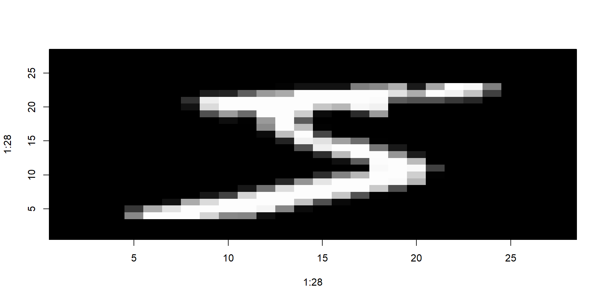
Digits
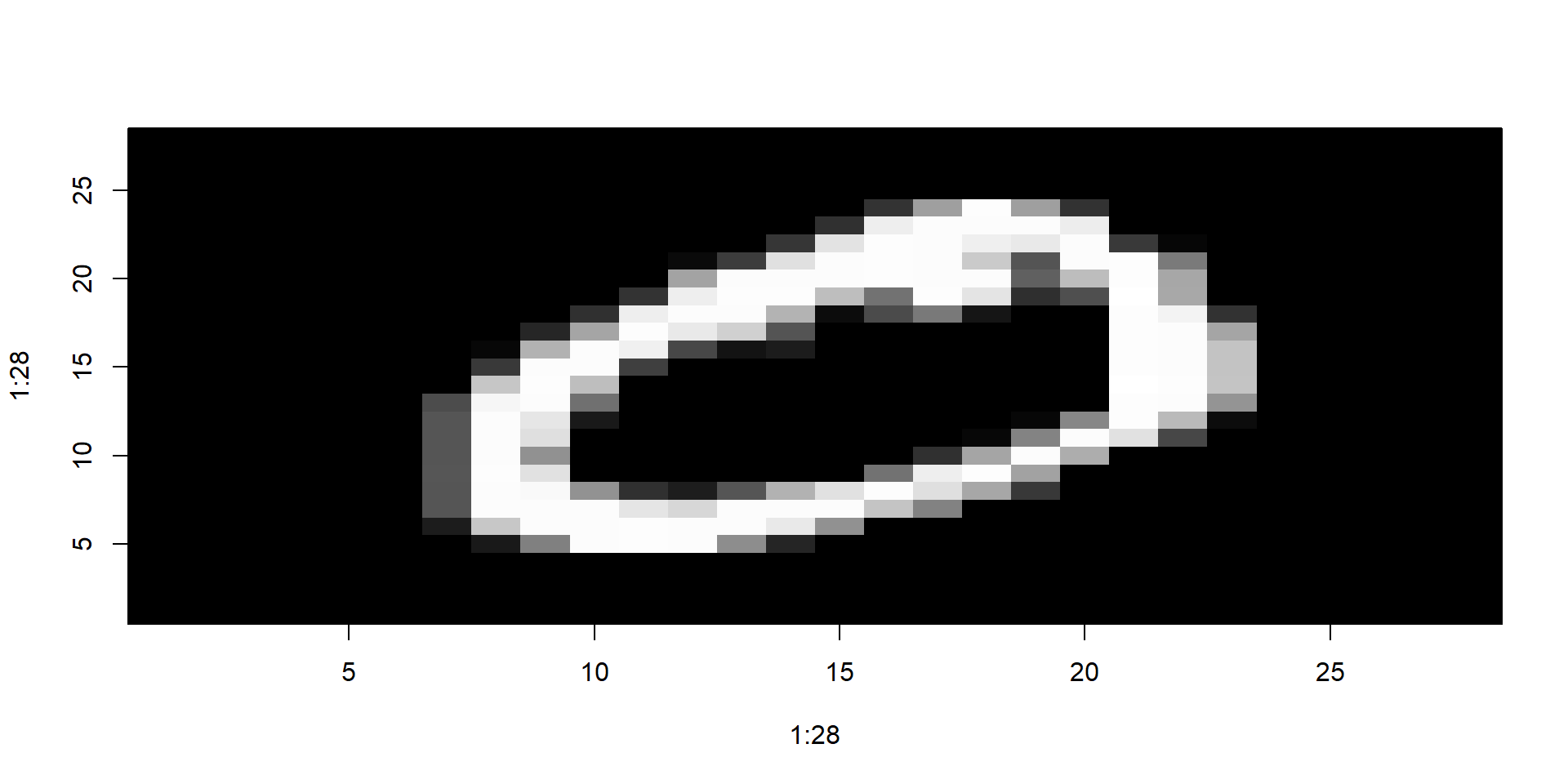
Digits
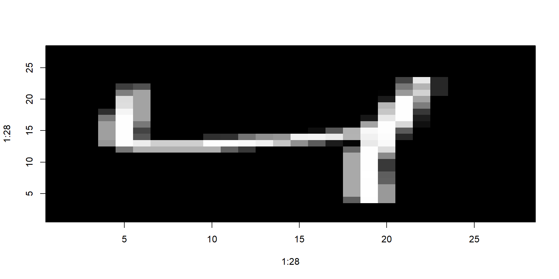
Digits

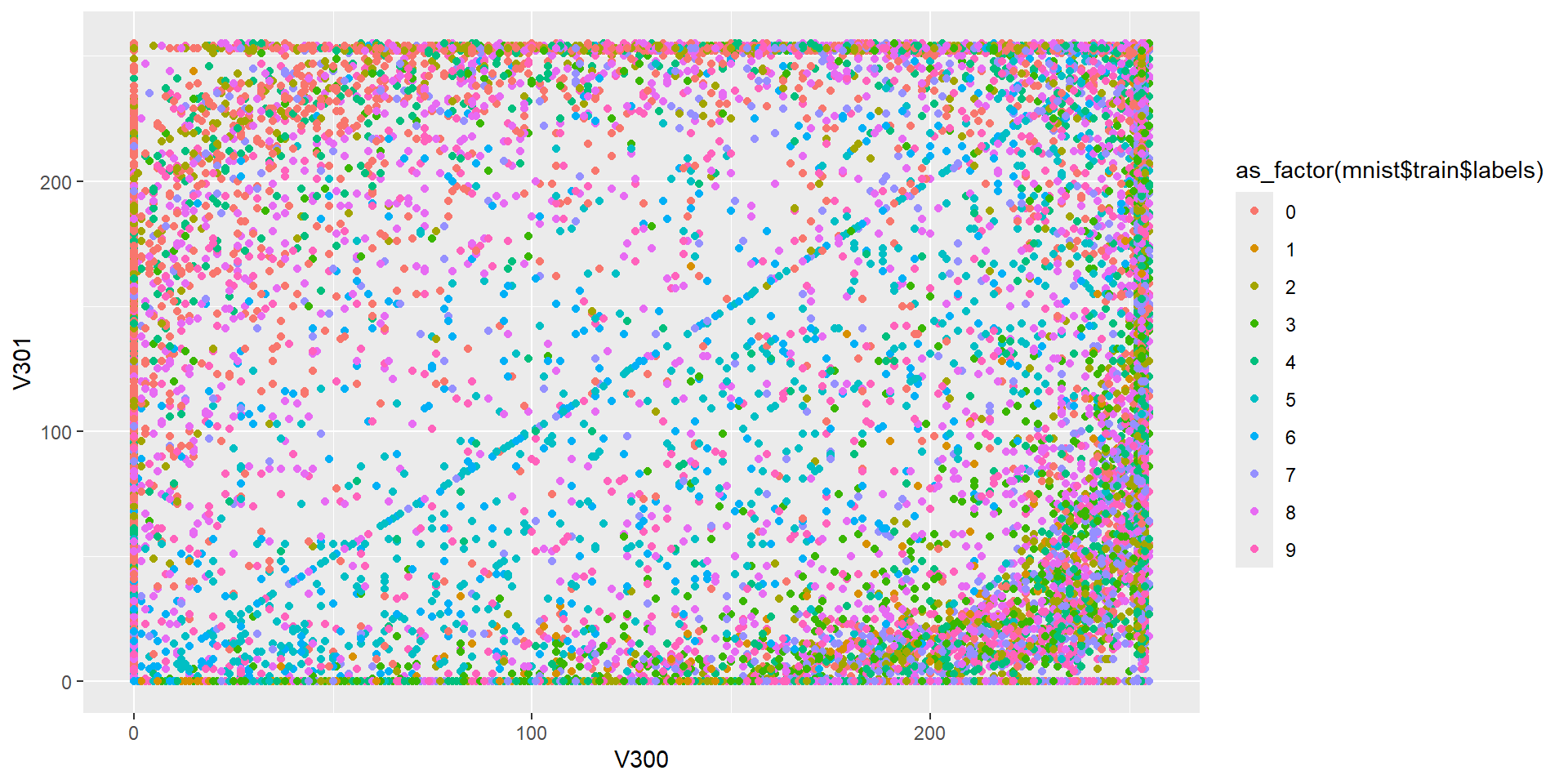
What if we want to visualize our data?
Unsupervised Learning & Dimensionality Reduction
- Unsupervised Learning: ML for unlabeled data (i.e. no response variables)
- Goal: Uncover patterns/structure within data
- Tasks:
- Clustering: finding sub-groups within our data
- Dimensionality Reduction: reducing the number of columns in our data set… why?
Dimensionality Reduction
- Goal phrasing 1: Reduce the number of columns, while losing as little information as possible
- Goal phrasing 2: Extract lower-dimensional structure from our data
- Analogy: file compression
Which One is Compressed?

Which One is Compressed?
Idea
- We managed to:
- Reduce file size by 70%
- Note lose much information
- Extract underlying structure (a duck)
Thinking about structure in tabular data
Underlying Structure
- What dimension is our data in?
- What is the underlying structure here?
- What is the dimension of a plane?
Visualizing Plane

Thinking about structure in tabular data
Underlying Structure
- What dimension is our data in?
- What is the underlying structure here?
- What is the dimension of a line?
Visualizing 2D
Visualizing 1D

Visualizing 1D Data
Thinking about structure in tabular data
Underlying Structure
- What dimension is our data in?
- What is the underlying structure here?
- What is the dimension of a plane?
Visualizing Plane

Discussion
- What’s the difference between the first two scenario’s and the third scenario?
- How much have we reduced the dimension?
- How much information have we lost?
Principal Component Analysis (PCA)
Vector’s and Projections
Basis Vectors and New Coordinates
- Plane above: \(z = x + y\)
- New Directions:
- New Direction 1: \(\vec{d}_1 = \langle 1, 1, 2\rangle\)
- New Direction 2: \(\vec{d}_1 = \langle 1, -1, 0\rangle\)
- New data:
- New \(x\): \(1\times x_{old} + 1\times y_{old} + 2\times z_{old}\)
- New \(y\): \(1\times x_{old} - 1\times y_{old} + 0\times z_{old}\)
- Note: Not quite correct, need to re-normalize
New Data
new_data <- data |>
  mutate(new_x = x + y + 2*z,
         new_y = x - y,
         new_x = new_x/6, #re-normalizing
         new_y = new_y/2)

new_data |> head() |> kable()| x | y | z | new_x | new_y |
|---|---|---|---|---|
| -0.5604756 | -0.9957987 | -1.5562744 | -0.7781372 | 0.2176615 |
| -0.2301775 | -1.0399550 | -1.2701325 | -0.6350663 | 0.4048888 |
| 1.5587083 | -0.0179802 | 1.5407281 | 0.7703640 | 0.7883443 |
| 0.0705084 | -0.1321751 | -0.0616667 | -0.0308334 | 0.1013418 |
| 0.1292877 | -2.5493428 | -2.4200550 | -1.2100275 | 1.3393153 |
| 1.7150650 | 1.0405735 | 2.7556384 | 1.3778192 | 0.3372458 |
What’s actually happening
- We are projecting each observation onto our new directions \(\vec{d}_1\) and \(\vec{d}_2\)
- Visualization
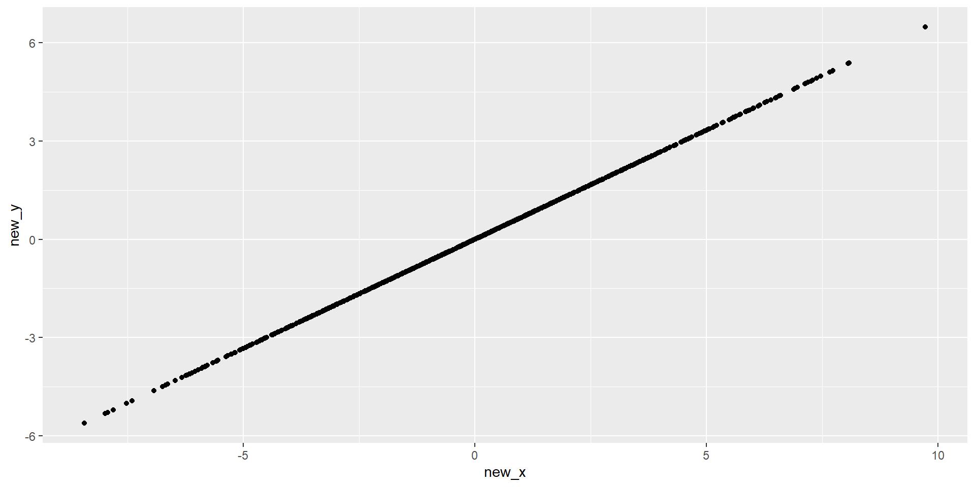
Projecting our data
Plotting these

Principal Component Analysis (PCA)
PCA Vocabulary
- Principal Component (PC1): direction in \(p\)-dimensional space (e.g. \(\langle 1, 1, 2\rangle\))
- Scores: our new variables (e.g. \((-0.56\times 1 + -0.996\times 1 + -1.56\times 2)/6 = -0.778\))
- Loadings: For direction above’
- Loading on \(x\) is 1
- Loading on \(y\) is 1
- Loading on \(z\) is 2
Recall: Variance
- What is variance?
- Intuitively: what does variance measure?
- Variance: \(\frac{1}{n-1}\sum_{i=1}^n(x_i - \bar{x})^2\)
- Average of the squared distance from zero of each observation
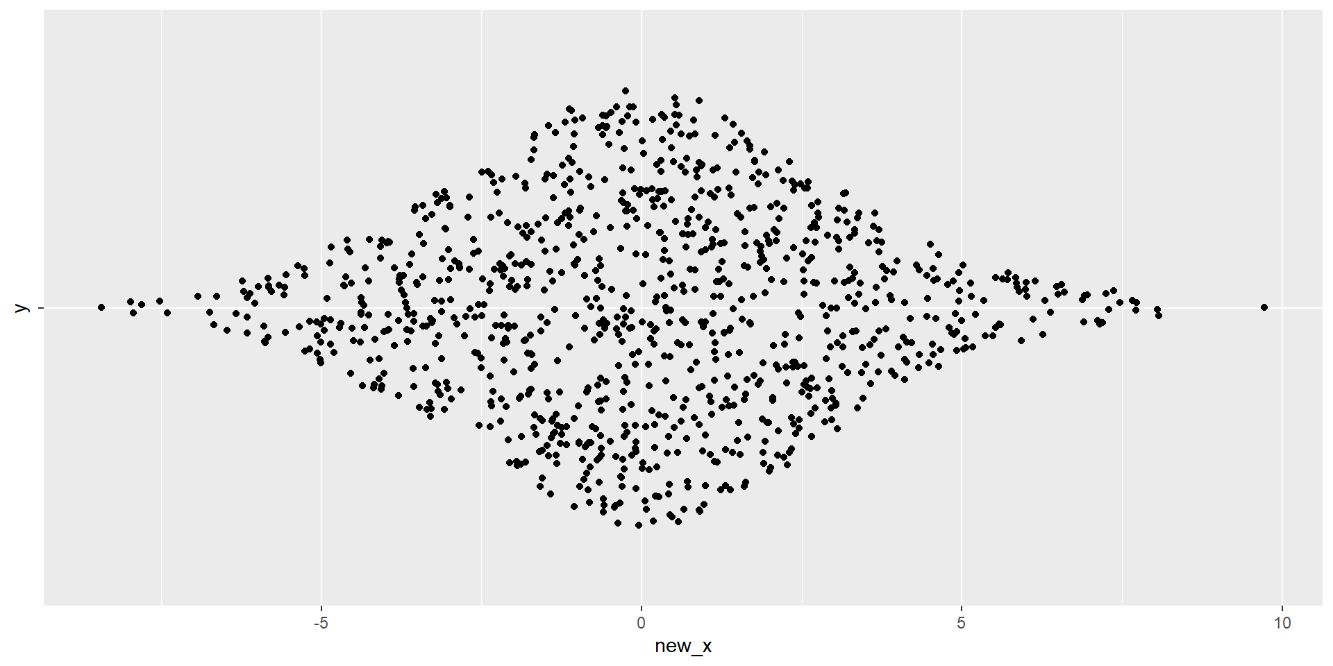
Idea behind PCA
- Select first PC so variance of scores is the maximum
- Iteratively:
- Select next PC so variance of scores is maximize AND new PC is orthogonal to all other PCs
- What does orthogonal mean?
Easy Example
- Exercise: What should the first and second PCs be?

How much variance is explained by each of the PC’s?
What proportion of variance is explained by each of the PC’s?
| name | value | proportion |
|---|---|---|
| var1 | 0.9834589 | 0.9391552 |
| var2 | 0.0637151 | 0.0608448 |
- 93% of our variance (information) is contained in our first PC
Harder Example
- Exercise: What should the first and second PCs be?

How much variance is explained by each of the PC’s?
Next Time
- Using R to apply this to bigger data sets
- More on interpreting PCA